Chapter 1: Data#
Note
This book is a work-in-progress! We’d love to learn how we can make it better, especially regarding fixing typos or sentences that are unclear to you. Please consider leaving any feedback, comments, or observations about typos in this google doc.
The log jam you don’t even know you’re stuck in will be broken by a shift in representation.
– Michael Sorkin, Two Hundred Fifty Things an Architect Should Know
1.1 Introduction#
Humans are visual creatures, and directed graphs leverage our visual perception and spatial thinking, by laying out all of the pertinent details in a single view. For example compare the textual description of the mythological romance in the last chapter aginst its description as a directed graph:
Mythological Romance:
Aphrodite loves Adonis and Adonis loves Aphrodite. But Adonis is polyamorous and is also in love with Narcissus. And Narcissus, of course, loves only himself.
Note how the written description requires concentration and parsing to understand. But the associated graph makes all the essential information instantly available.
Directed Graph
When we look at a directed graph we can instantly see many relationships: this arrow is connected to these vertices, this vertex has no arrows, etc. Such implicit relationships are made apparent by the visual proximity of the graph elements. But unlike humans, computers are not visual creatures. If we want to involve a computer in our thinking we need to find another (non-visual!) way of communicating these relationships. The following video outlines one possible approach to redescribing our graph in a way that a computer can understand.
1.2 Source and Target Maps#
The virtue of making these relationships explicit is that the information can now be written in list form, and lists are a data structure that can be easily typed into a computer (using Algebraic Julia).
DISCLAIMER: In our code samples we will be working with a graphics visualization tool called Graphviz. This is a convenient visualization package for our “under development” software of Algebraic Julia, but it can sometimes behave like an inept reconstructor. Don’t be surprised if, along the way, Graphviz gives you some puzzling representational choices!
Puzzles#
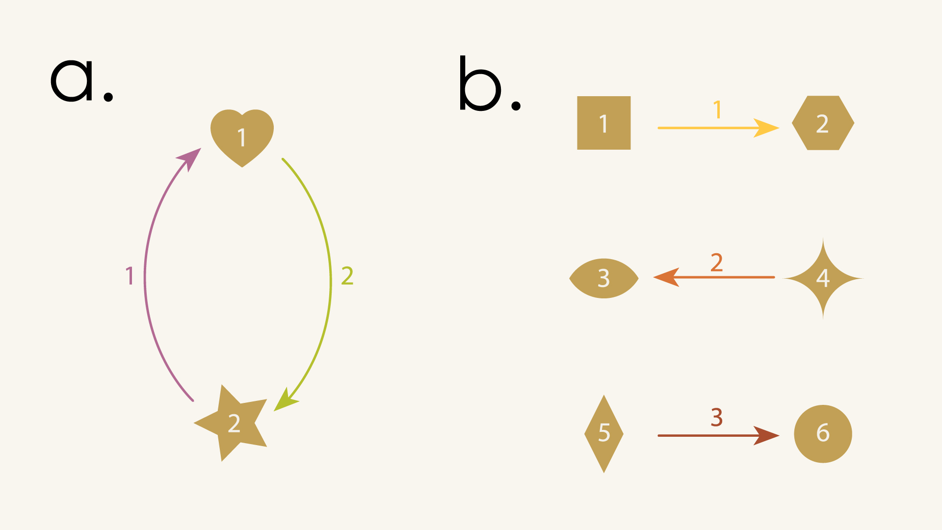
Puzzle 1
Can you draw the directed graphs described by these source and target maps on a paper?
a.
b.
Puzzle 2
Examine the following directed graphs. Can you draw their source and target maps?
Puzzle 3
Convert the source and target maps from the last problem into lists of numbers.
Puzzle 4
Coding time!! The Introduction chapter explains How to edit and run the code
Take your lists of numbers from the last problem and enter them into the code below – replace the ‘?’s under “src” and “tgt”. Run the code . Do the graphs look the way you expected?
using Catlab.CategoricalAlgebra, Catlab.Graphs, Catlab.Graphics

AJ_Problem4a = Graph()
add_vertices!(AJ_Problem4a,2)
add_parts!(AJ_Problem4a, :E, 2, src=[?,?], tgt=[?,?])
to_graphviz(AJ_Problem4a)
AJ_Problem4b = Graph()
add_vertices!(AJ_Problem4b,6)
add_parts!(AJ_Problem4b, :E, 3, src=[?,?,?], tgt=[?,?,?])
to_graphviz(AJ_Problem4b)
1.3 On the importance of finding the right abstractions#
We’ve come up with one way to describe a directed graph to a computer. But is it the best way? Are there other approaches we should consider?
In our current approach each arrow gets assigned a unique source vertex and a unique target vertex. What would happen if we flip the direction of that assignment? That is, instead of the assignment starting from the arrows, we instead start from vertices, assigning each vertex as a source or target to the arrows.
 What does it mean when connections flow in opposite directions?
Is there a difference between “arrows-first” and “vertices-first” representations?
At first glance, these might seem like the exact same thing. But in fact, a whole bunch of problems arise if we try to think about directed graphs in the second way!
First of all, there are many directed graphs that can’t be expressed this way at all - at least not without relaxing some of our rules for making source and target maps.
In the above graph, some vertices need to map to many arrows while others don’t map to any. So instead of the simplicity we had in the arrows-first approach (where each arrow had one-and-only-one source vertex and one-and-only one target vertex) we now must allow for arbitrary of branching in our maps. This looser specification gives rise to a number of bookkeeping headaches. For example, how you would express the above map to a computer? Lists won’t do it anymore. It turns our you’ll now have to enter lists of lists!
But more importantly, the vertex-first approach makes us vulnerable to the DANGLING EDGE CONDITION.
Suppose we created a random graph using the vertices-first approach, just throwing together source and target maps, arbitrarily connecting things without giving any thought to what the resulting graph will be like.
 “Random” source and target maps
In this case, when we try reconstruct the graph from this random data, we get a mutant!
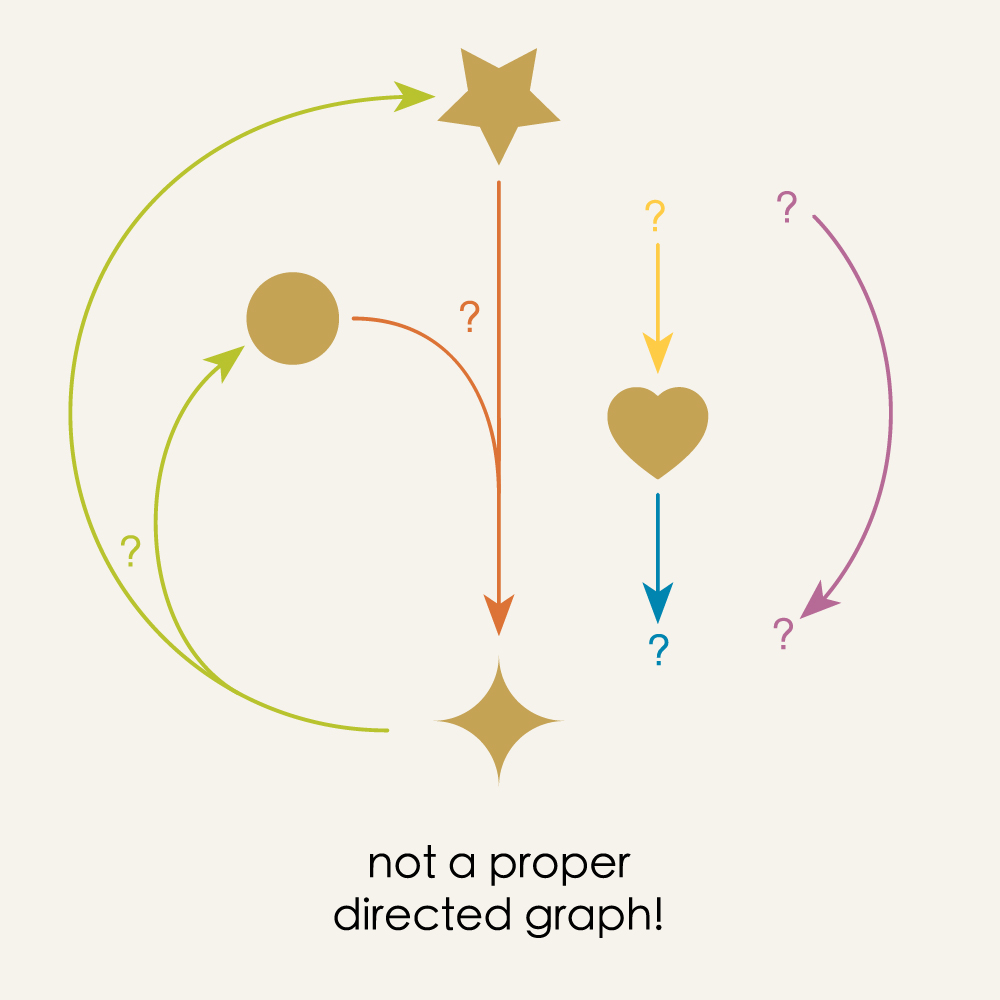
Dangling arrows, arrows that have to come out of multiple vertices somehow, arrows floating off by themselves unattached to anything. It’s carnage! By designing our maps in the vertices-first approach we open up the possibility of creating nonsense: maps which may appear valid at first, but which produce broken directed graphs when we try to interpret them. By contrast, any maps in the arrows-first approach can’t help but be proper directed graphs.
Pause and Ponder!
Why is this?
Can you think through why arrows-first is always “safe”, while vertices-first can produce the DANGLING EDGE CONDITION?
Our purpose in comparing these approaches is to highlight the difference between “good” and “bad” representations. It’s hard to escape the feeling that the arrows-first approach is somehow the natural way to describe directed graphs. There is an exact correspondence between what we’re interested in (directed graphs!) and what the maps are capable of expressing. By contrast, the vertices-first approach produces the typical problems of “bad” representations, which force you to countenance nonsense and deal with problematic edge cases. In a word, they’re fussy. And this kind of fussiness is not just annoying, it turns out to be a barrier to abstraction.
As we go through this book we will take a series of increasingly abstract points of view on graphs. The beauty of beginning this journey with a good representation is that it permits us to move up the ladder of abstractions cleanly, at each stage fully disregarding the details of the previous level and being able to take for granted that everything below our current view will naturally take care of itself.
1.4 Summary#
In this chapter we have moved up our first rung on this ladder of abstractions - from directed graphs themselves to the graph data. In the coming chapters we will continue to climb, moving on to “Blueprints” in Chapter 3 and “Categories” in Chapter 4. At each step, we will obtain new capabilities and new ways of thinking about structures and modeling. But as we will see, we’re only able to reap the cumulative benefits of abstraction because we’re choosing the more elegant representation at the start.