Chapter 3: Blueprints - Part I#
Note
This book is a work-in-progress! We’d love to learn how we can make it better, especially regarding fixing typos or sentences that are unclear to you. Please consider leaving any feedback, comments, or observations about typos in this google doc.
3.1 Introduction#
We have now seen how directed graphs can be useful for modeling the world. However, in some situations they’re not actually the best choice.
Suppose we were making a directed graph to represent the social network on TikTok:
Vertices are people
Arrows are “follows” – going from a person to someone they follow.
A piece of our graph would look like this:
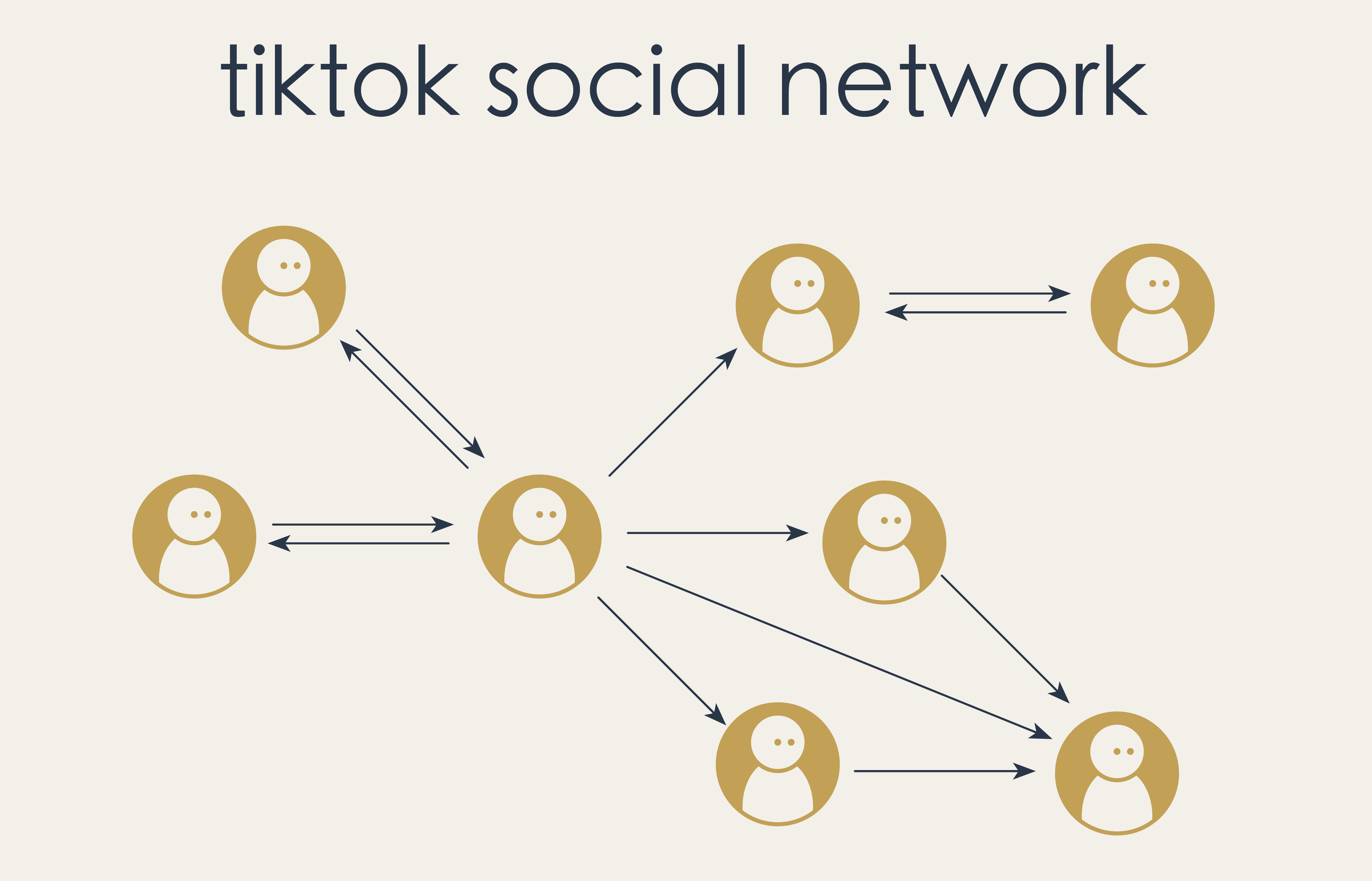
In this case, directed graphs are the perfect choice for modeling the social network because TikTok follows are directional. Someone you follow may not follow you back.
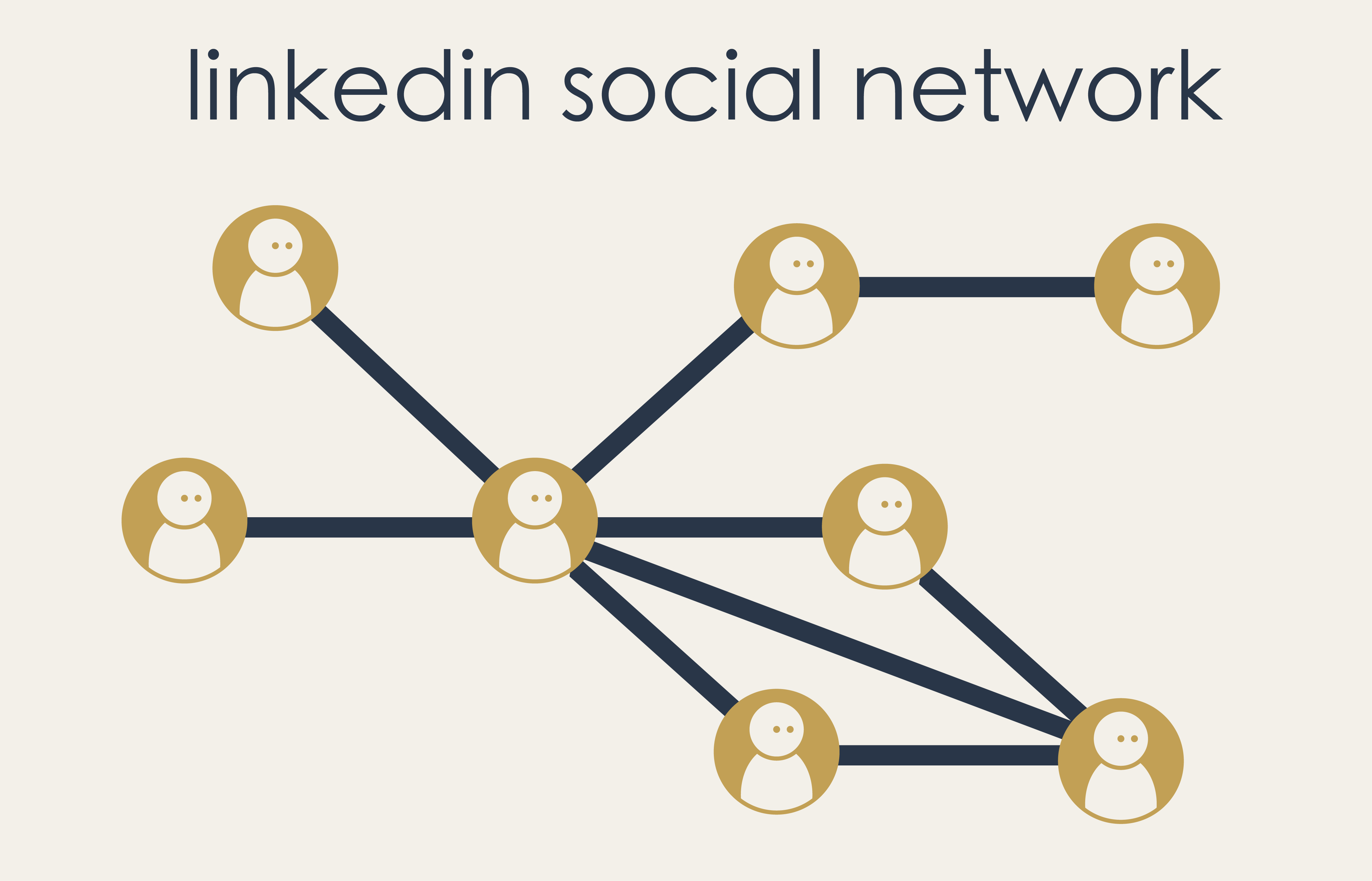
Now let’s imagine doing the same thing for connections on LinkedIn. In this social network, both parties must mutually agree to the connection. So a LinkedIn connection is symmetric, not directional.
To model this kind of social network we need a different kind of graph. We call these “undirected graphs” and, as the name surely suggests, these are like directed graphs but with non-directional edges connecting the vertices.
Pause and Ponder!
How would you represent an undirected graph in terms of source and target maps?
Undirected graphs are just one example from a whole zoo of different kinds of graphs we might want to model with. In this chapter we’ll look at a few specimens from this zoo.
In the process, we’ll develop a versatile and flexible approach for representing many different kinds of graphs in a computer using AlgebraicJulia.
3.2 Introducing Blueprints#
Chunky arrows#
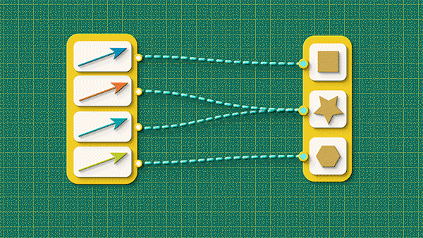
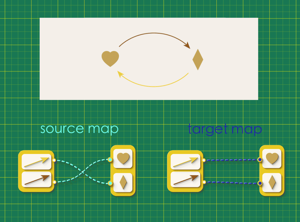
We’ll begin this chapter with a little tidying up. The basic building block we’ve been working with so far is a map, a bundle of connections in which every item on one side gets connected to some item on the other. For example:
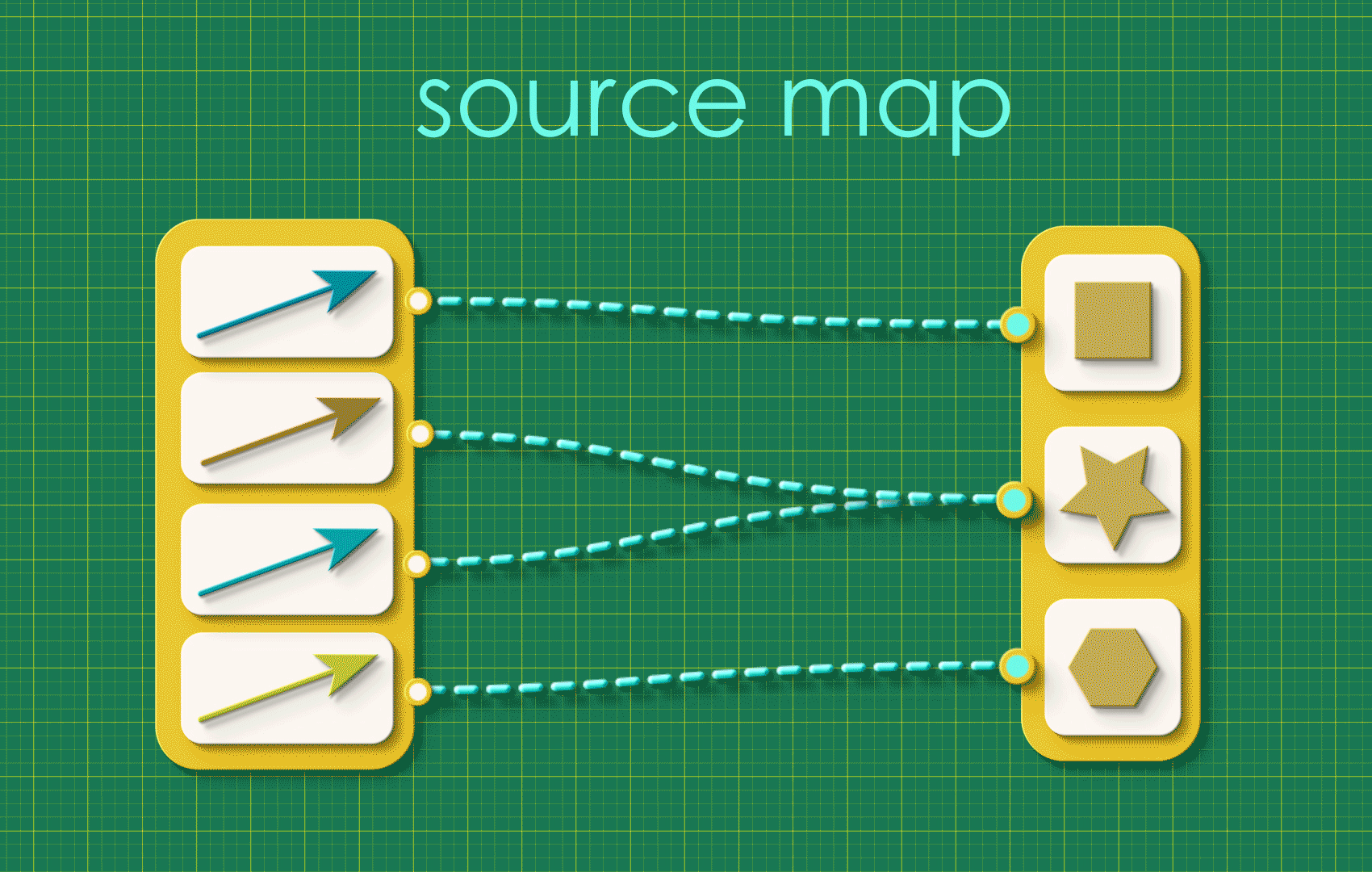
Source and target maps can be a little busy looking so we’re going to simplify our view! Let’s introduce a new abstraction that hides all of this detail. We’re going to:
wrap these connections in one big tube
put an arrow point on this tube so we can remember which direction the connections were going
wrap the items at either end in labelled spheres
and forget all about those underlying details!
A big chunky arrow like this is easy to draw and easy to think about. Whenever we see one we can take for granted that there is some specific set of connections bundled up “under the hood.” This is just like in an algebra equation where, when we see the variable ‘x’, we know it is a placeholder for a number. Chunky arrows are like the variables for maps.
Directed graphs using chunky arrows#
Can we represent a directed graph using these chunky arrows? Recall that a directed graph is defined by two maps, both of which connect the same collections of arrows and vertices.
Instead of representing these maps side by side like this, let’s combine them so that they run in parallel. When wrapped in chunky arrows these connections will be in the following configuration:
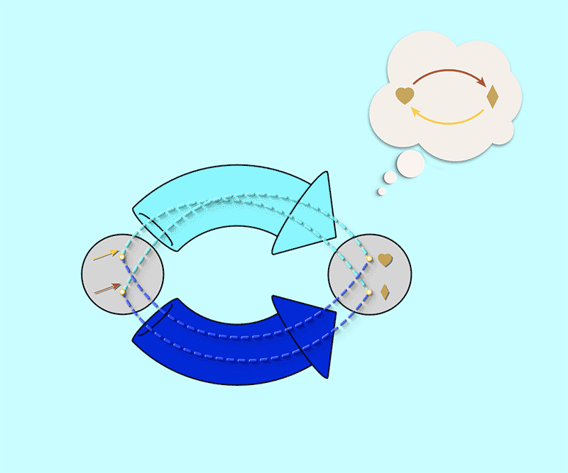
Such a pair of parallel maps is the blueprint of all directed graphs. Any easy way to think about a blueprint is like a form to be filled. The form has placeholders for the data that is required – for example, Firstname, Lastname, and so on. Simiarly, a blueprint of a directed graph is a fillable form for a directed graph. The word schema is the relational thinking term for blueprints. These are not just any blueprints, but blueprints for building mathematical objects, for example, directed graphs.
Schema is the relational thinking term for blueprints.
We generally draw the schema for directed graphs as two arrows marked src and tgt.
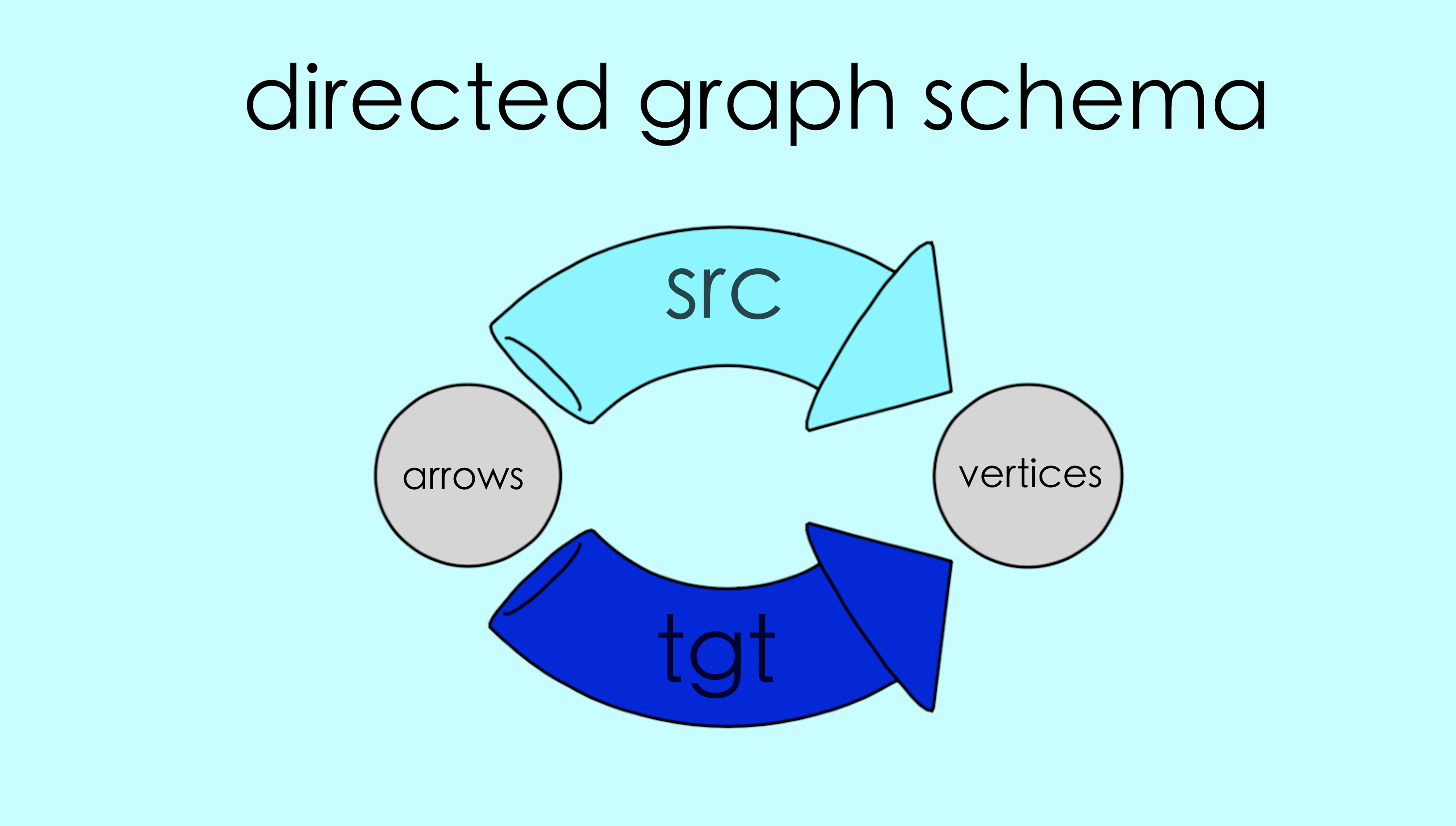
Any particular pair of maps in this configuration is said to be an “instance” of this schema. By filling in the schema in different ways we create different instances, and every instance corresponds to some directed graph.
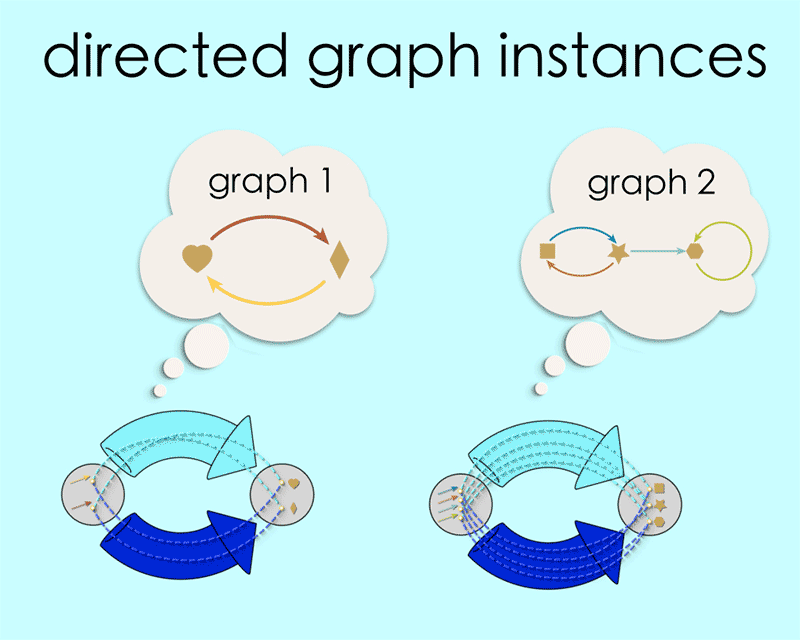
You may have noticed that our blueprint is itself a directed graph! This is where things get interesting! This means we can input the schema to a computer in AlgebraicJulia using the concept of source and target maps, as we learned about in Chapter 1.
In the code below we use A for arrows, V for vertices, and define them as Objects. Hom(X,Y) is AlgebraicJulia syntax meaning a “chunky arrow from X to Y.” We use it to define the source and target of the chunky arrows src and tgt.
@present Graph(FreeSchema) begin

  V::Ob
  A::Ob

  src::Hom(A,V)
  tgt::Hom(A,V)

end
And that’s how AlgebraicJulia sees a directed graph to be!
3.3. Summary#
In this chapter, we abstracted the information of a single directed graph and created schema of all directed graphs.
This general characterization of all directed graph using blueprints is quite a powerful and versatile idea as we will see. This notion of schema will provide the foundation for relational thinking (using a mathematical object). Let us continue our journey of schema in the next chapter where we we will next see how we can add to the schema of directed graphs to describe other kinds of graphs, and also other cool mathematical objects beyond graphs.