Chapter 5: Categories#
Note
This book is a work-in-progress! We’d love to learn how we can make it better, especially regarding fixing typos or sentences that are unclear to you. Please consider leaving any feedback, comments, or observations about typos in this google doc.
Attention
We have reached the shores of relational thinking!
5.1 Introduction#
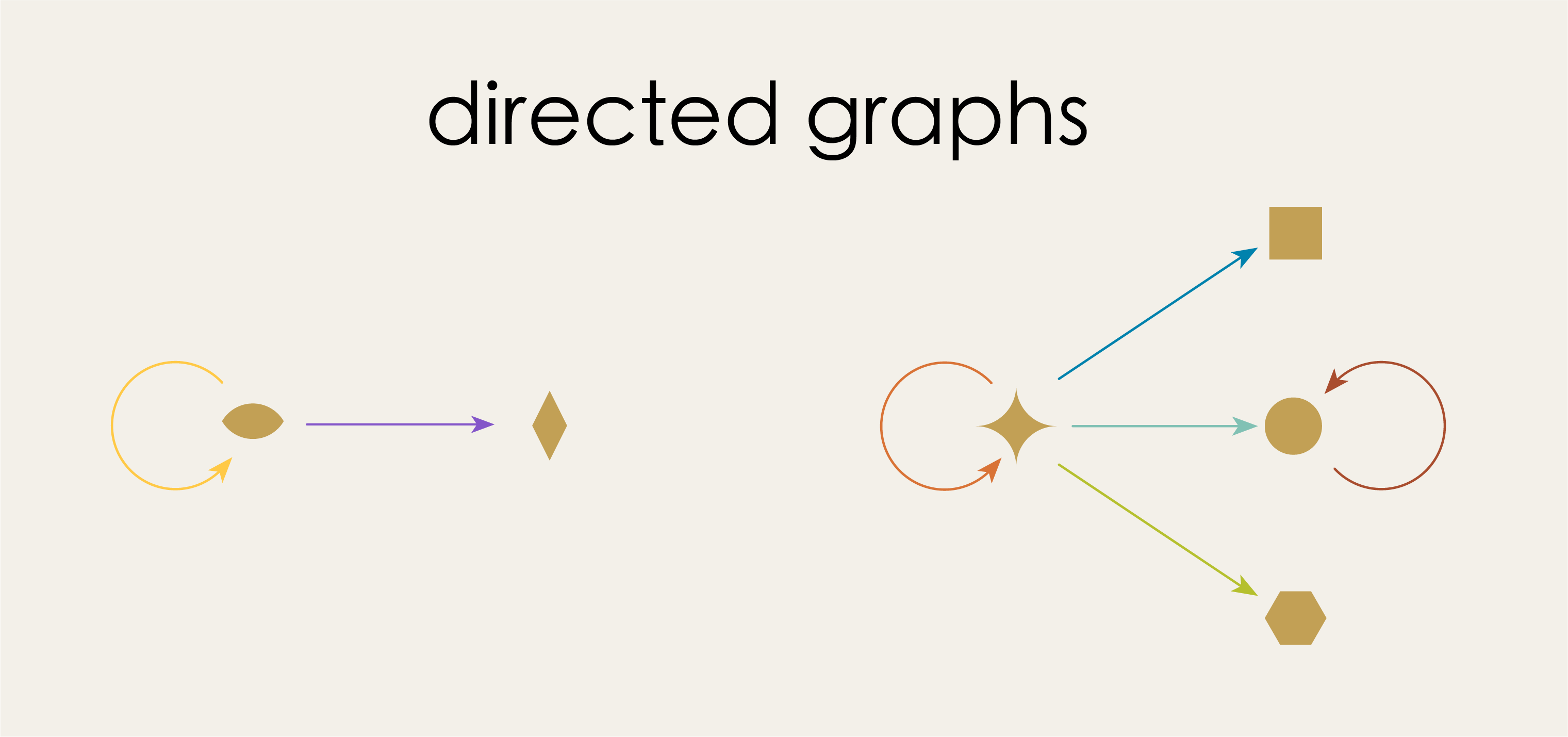
In the last chapter we encountered different schemas for different kinds of graphs.
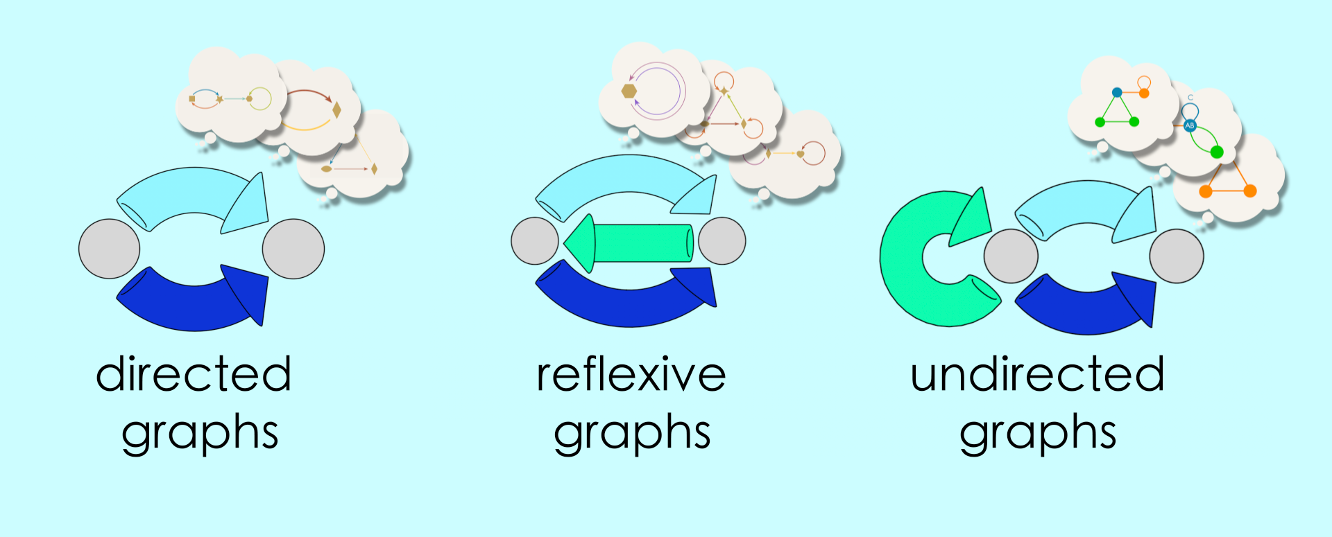
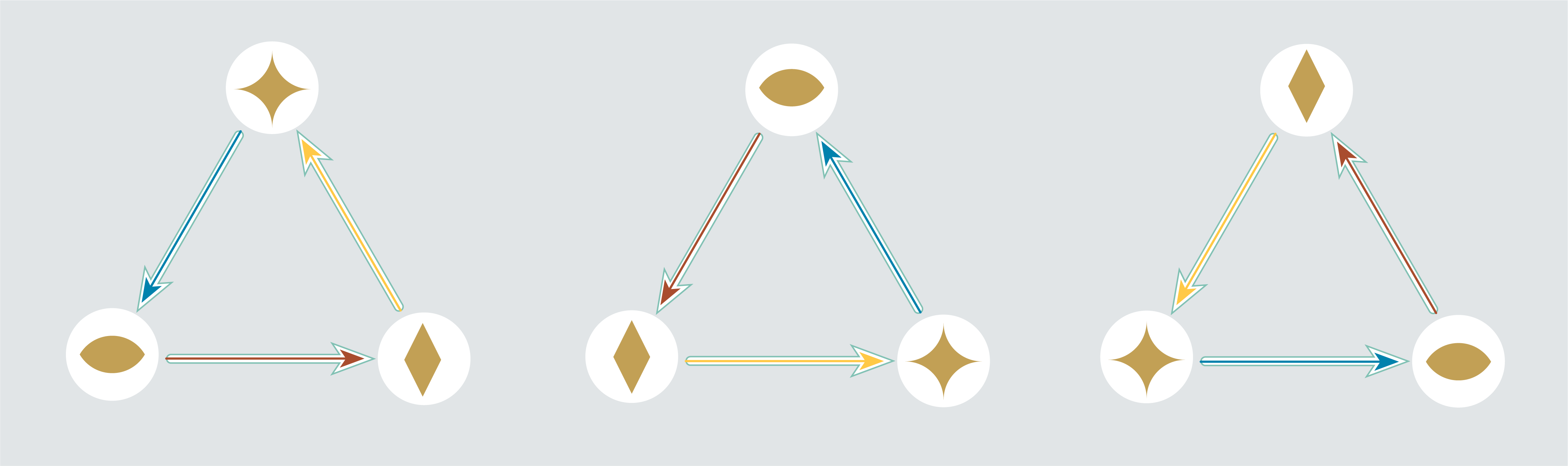
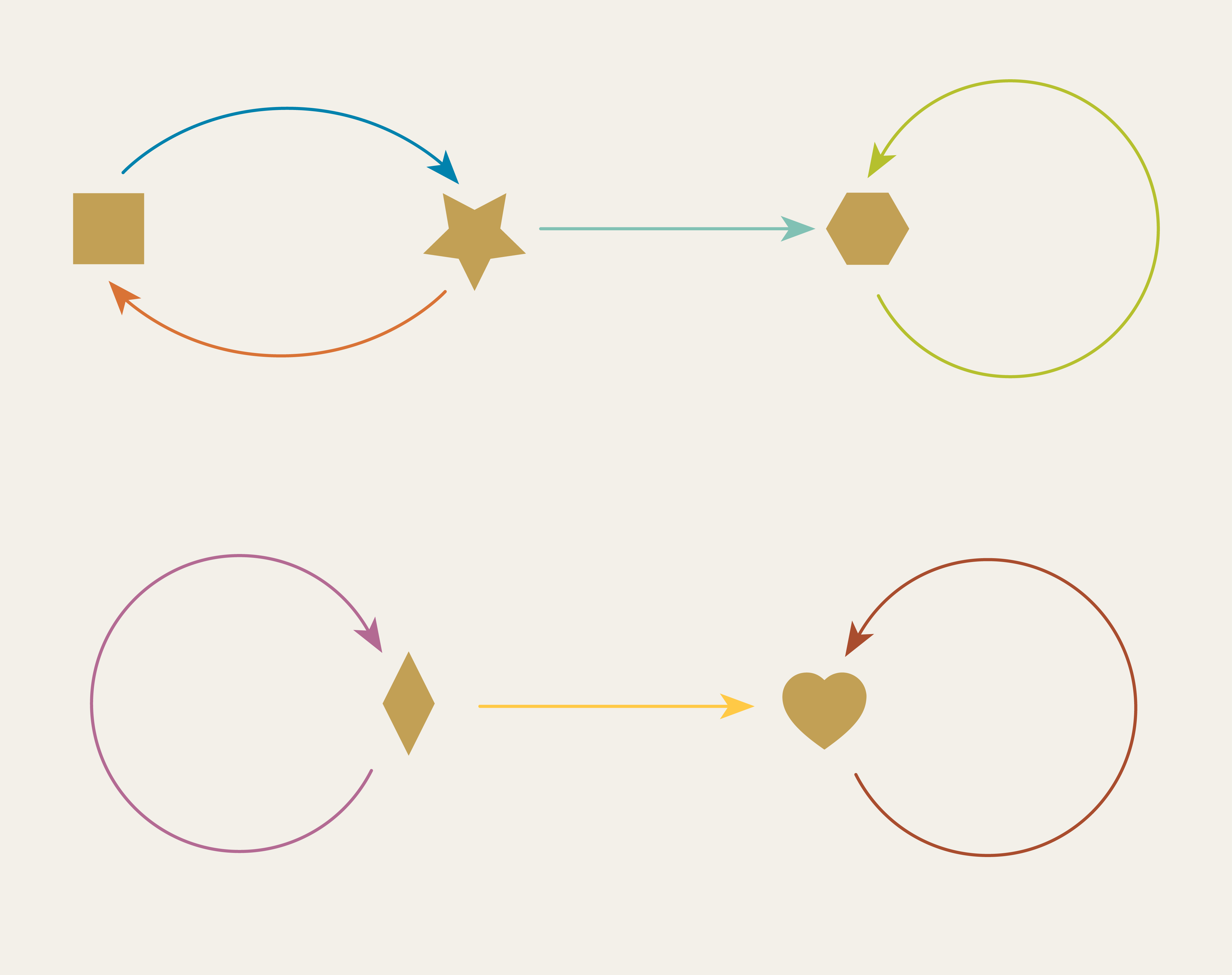
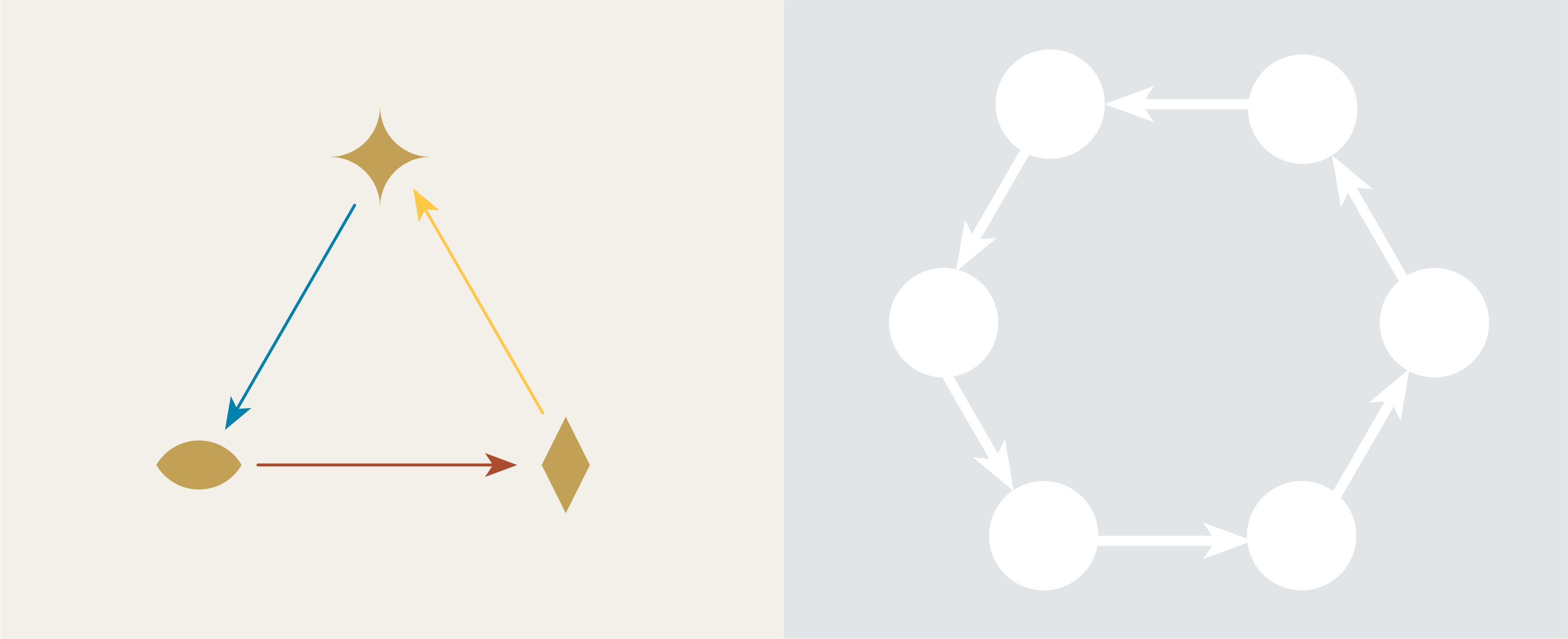
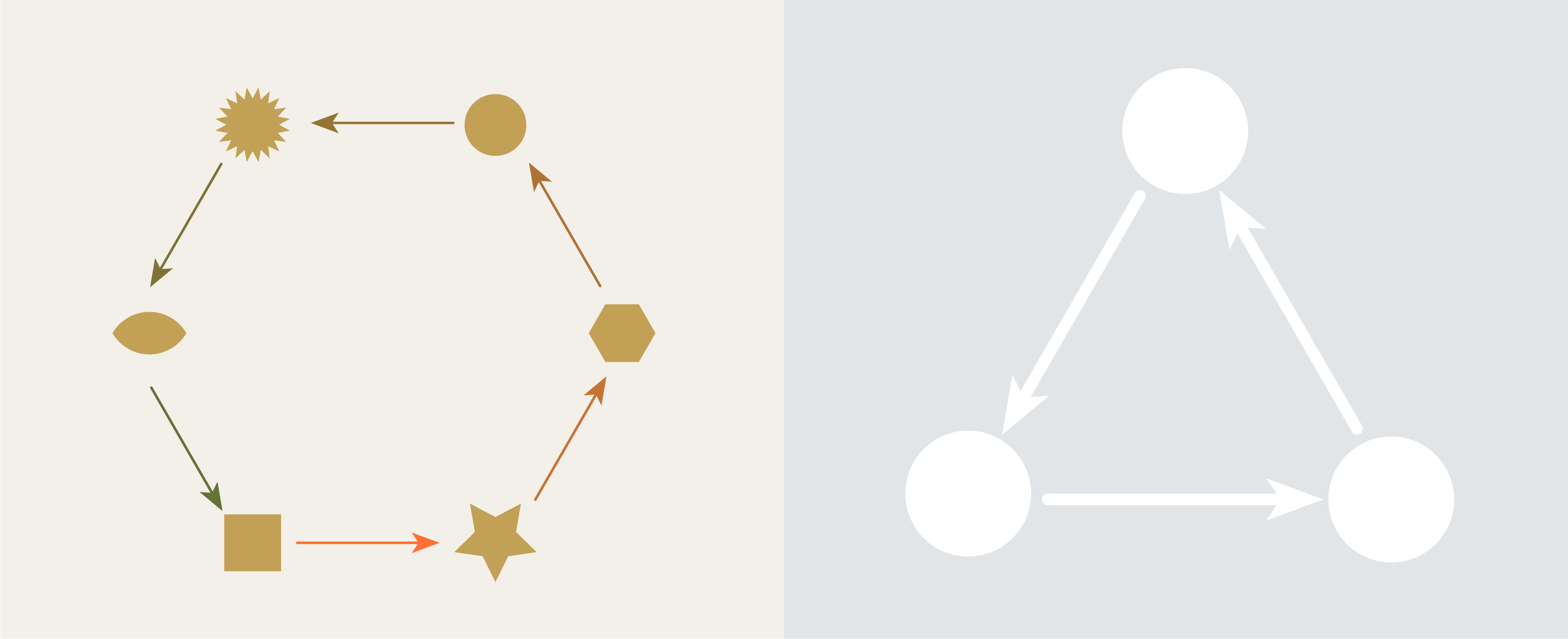
Given a schema such as the ones above, there are infinite number of graphs that each schema can generate. Each generated graph is called an instance of the schema. The above picture shows three instances for each schema. While it isn’t practical to specify every possible instance of a graph schema, it is practical to imagine a universe that has all possible instances floating in space, one endless swarm of things the schema refers to. (No, we do not ask what those instances are.)
How boring a universe will be if each one of its objects just exist by itself with no connection to another object like the endless swarm of things above? Richness and complexity arises from connections. Our physical world is incredibly rich and complex because of the relationships between individual things.
Attention
So our goal for this chapter is to say what does it mean for two graphs to be related!
Once we achieve this goal, our description of a universe generated by a schema will be complete – a universe has objects and relationships. In relational thinking terms, universe (generated by a schema) is called a category.
Completing this goal will move us up to the fourth and the topmost rung in our ladder of abstractions, from schemas (blueprints) to categories. 🚀
5.2 Graph Injections#
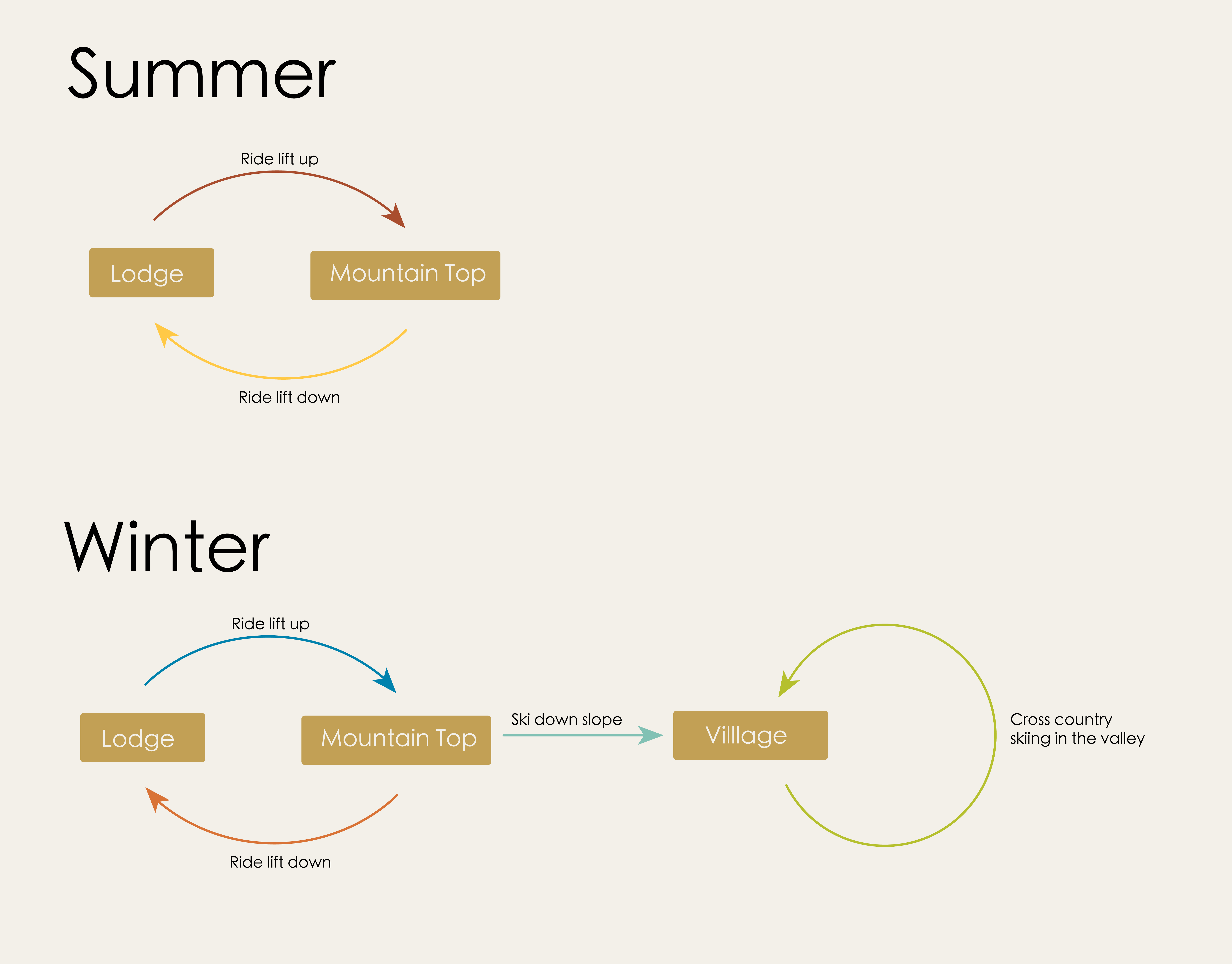
Can you recollect from chapter 0 the directed graph we drew for the layout of a ski resort? In winter, the visitors of this resort can ride the ski lift up and down the mountain, or ski from the top of the mountain to a village in the valley. 🏂
But suppose we visit this ski resort in the Summer when there’s no snow. At this time of year the resort lets guests ride up and down the mountain in the lift (which provides a lovely view!), but there is no way to get down the mountain into the village without a snow pack to ski on.
Let’s compare the summer and winter maps for the ski resort.
Point to ponder
How are these graphs related?
Graph injections, concretely#
One way to think about the relationship between the winter and the summer graphs is that we can turn one into the other. Given the Summer map I can turn it into the winter map by adding the additional vertices and arrows associated with travelling to the village. On the other hand, given the Winter map, I can create the Summer map by deleting the arrows and vertices associated with the village.
This is what we might call a “procedural” way of thinking about the Summer and Winter maps; you imagine step-by-step procedures that could be applied to transform one map into the other. In order to make our way towards “relational” thinking we are going to recommend different way of looking at these two graphs.
Note how the Summer graph is basically contained inside of the Winter graph. For the Summer graph to be a “part” of the Winter graph means, in effect, that we can map the vertices of the Summer graph into the vertices of the Winter graph, and the arrows of the summer graph into the the arrows of the winter arrows, as in the picture below.
We call this a “graph injection”. “Summer graph” is the graph which was injected. “Winter graph” is the graph which received the injected graph.
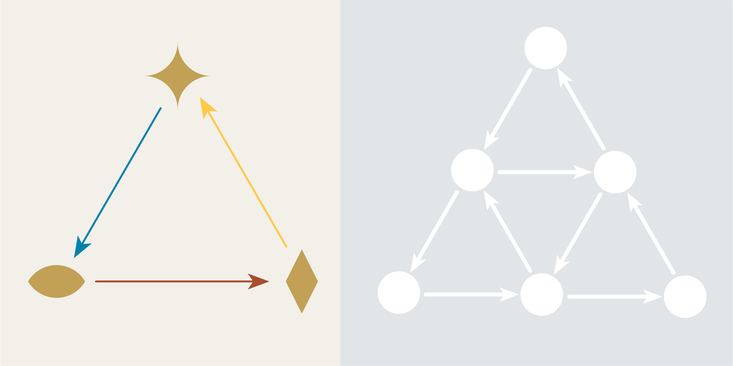
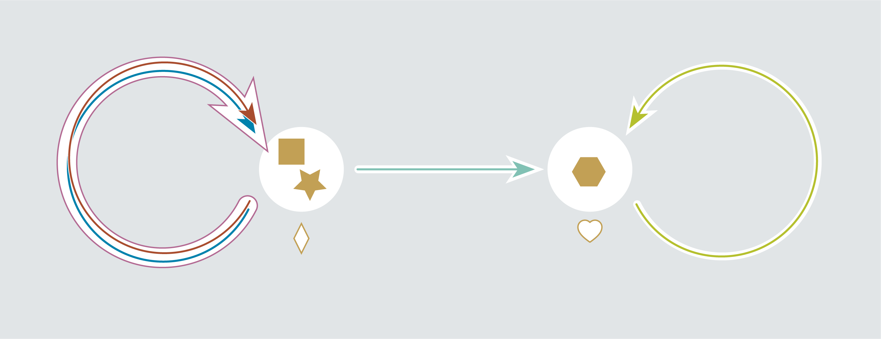
In order to visualize injections clearly let’s introduce some new visuals. Let’s redraw the vertices and arrows of the receiving graph to be white outlines, and move the colors and shapes out of the way.
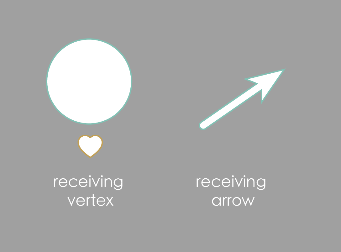
These outlines will “receive” the components of the injected graph. The process of placing the injected graph inside of the receiving graph can now be visualized like this:
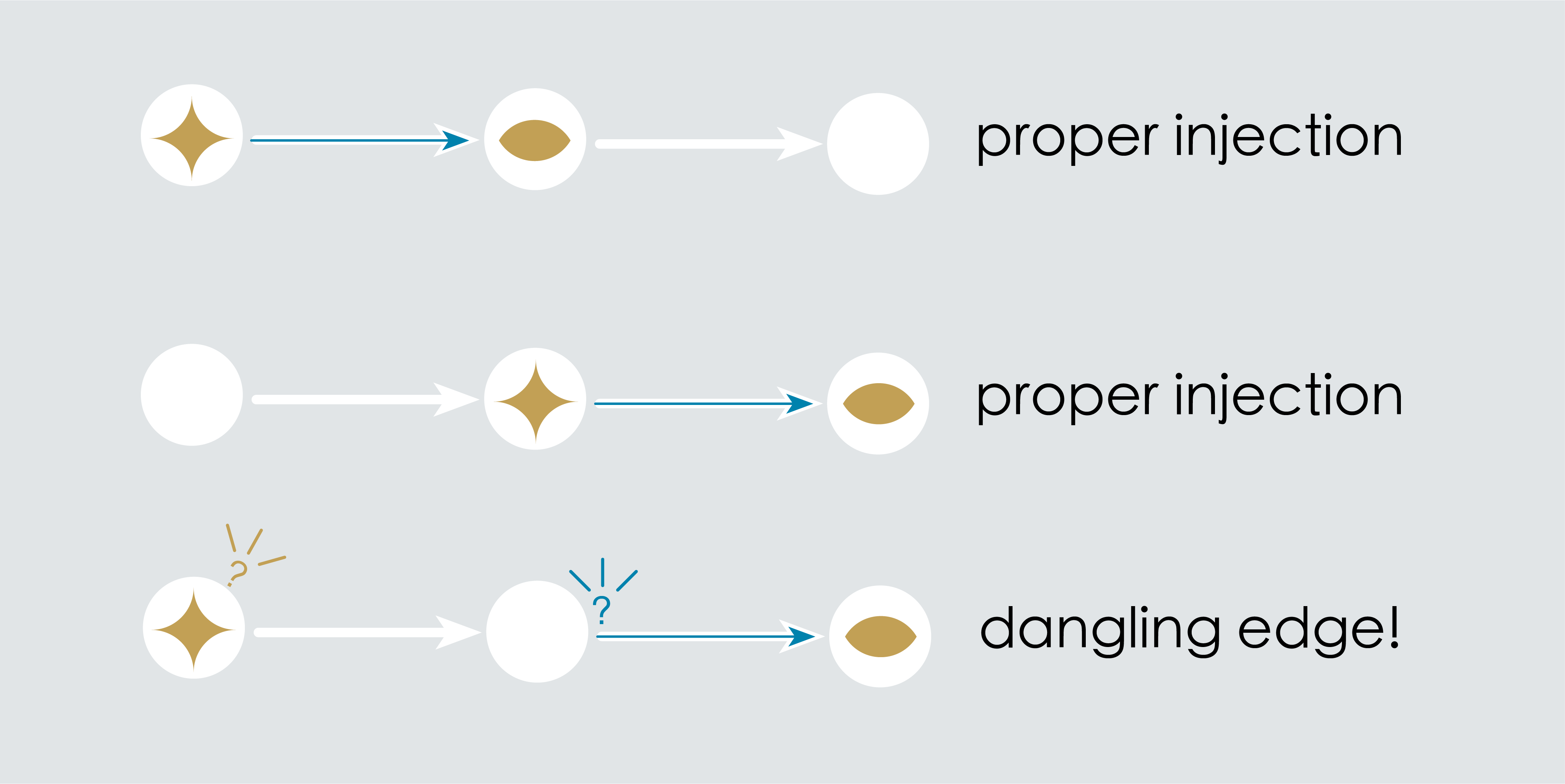
The final result gives us an complete picture of "what went where" in our injection. We sometimes call this the "image" of the first graph in the second.
CAUTION: An important detail about graph injections is that a graph is not allowed to come apart when getting injected. All arrows must stay attached to their source and target vertices through this process in order to avoid the DANGLING EDGE CONDITION and preserve the integrity of any underlying model.
Puzzles#
Puzzle 1.
How many ways can you inject the graph on the left into the graph on the right?
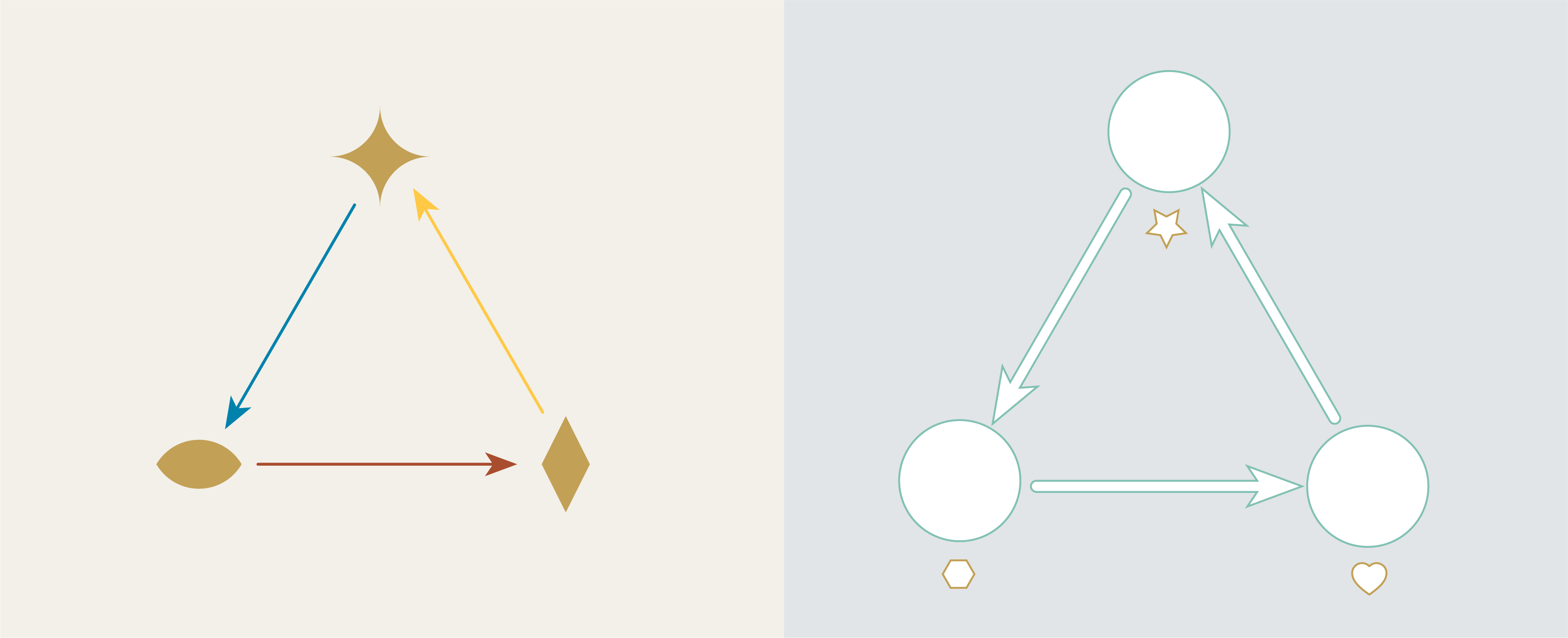
Puzzle 1 Solution:
The first graph can be injected in three different orientations.
Puzzle 2.
How many ways can you inject the graph on the left into the graph on the right?
Puzzle 2 Solution:
Twelve?
Pause and Ponder!
What strategies did you use to count the injections? Were you systematic or did you do it through trial and error? Could you design an algorithm (procedure) that a computer could use to solve these problems for you?
Graph injections as data#
Now that we have visualized graph injections in rung 1, we would like to how to represent a graph injection as data in Rung 2. Remember, humans are visual creatures, however computers are not!
We can actually capture all of the important details with a pair of maps. The first is a “vertex map”, connecting each vertex in Graph 1 to the vertex in Graph 2 where it lands. The second is an “arrow map” which connects each arrow in Graph 1 to the arrow it lands in Graph 2.
These two maps capture all the relevant information about the injection.
How to avoid dangling edges in the data?#
Recall our DANGLING EDGE CONDITION: For these pair of maps – vertex map and arrow map – to represent a proper injection of Graph 1 into Graph 2, the arrows of the injected graph have to stay attached to their respective source and target vertices.
Pause and Ponder
Under what condition(s) will the pair of maps keep Graph 1 intact when injecting into Graph 2?
We welcome the reader to ponder over this question using an arrangement as one shown below. The arrangement shows the source maps for Graph 1 and Graph 2 running horizontally and the “arrow map” and “vertex map” running vertically:
Pause and Ponder!
Starting from the top left corner of the square, let your eyes follow the dashed lines around the figure. Do you see any “patterns” in this system of connections?
Note how the dashed lines seem to flow “out” from the the top left and flow “in” to the bottom right. Starting from any arrow in the top left, there are two paths you can take around this square: an upper route and a lower route. Let’s focus on a specific arrow and consider what these routes “mean”. (We’ll label the endpoints as “A” and “V”)
Upper route
(The arrow must be brown in color. Our animator has been missing lately, so we have not corrected the color below.)
Reading across the top we have that the brown arrow has the heart vertex as its source. Reading down the right side we see that the heart gets sent to the square vertex in Graph 2. So the square vertex is “the vertex that receives A’s source.”
Lower route
Reading down the left side, we see that the brown arrow from Graph 1 gets sent to the blue arrow from Graph 2. The blue arrow is the image of A. Reading across the bottom we see that the blue arrow has the square vertex as its source. So the square vertex is “the source of the image of A.”
To complete the picture, let’s now revisit to our DANGLING EDGE CONDITION. “Coming apart” means, literally, that a vertex and an arrow that were connected in Graph 1 are not connected when they land in Graph 2. Suppose an arrow gets separated from its source by an attempted injection. For that arrow, the two routes around the square will look something like this:
That is, what it “means” for a graph to get broken is precisely that “the vertex that receives A’s source” is different from “the vertex that is the source of A’s image.”
So we can actually DEFINE a graph injection with a closed loop condition: starting from any arrow in the top left, the paths going either way around the square will always form a closed loop. In relational thinking terms, closed loop conditions are also called as commutativity conditions.
The closed loop condition applies to the target maps too. All together, this is the complete set of “data” describing the injection:
Going up a level of abstraction to Rung 3, a schema that describes a graph injection in general looks as shown below:
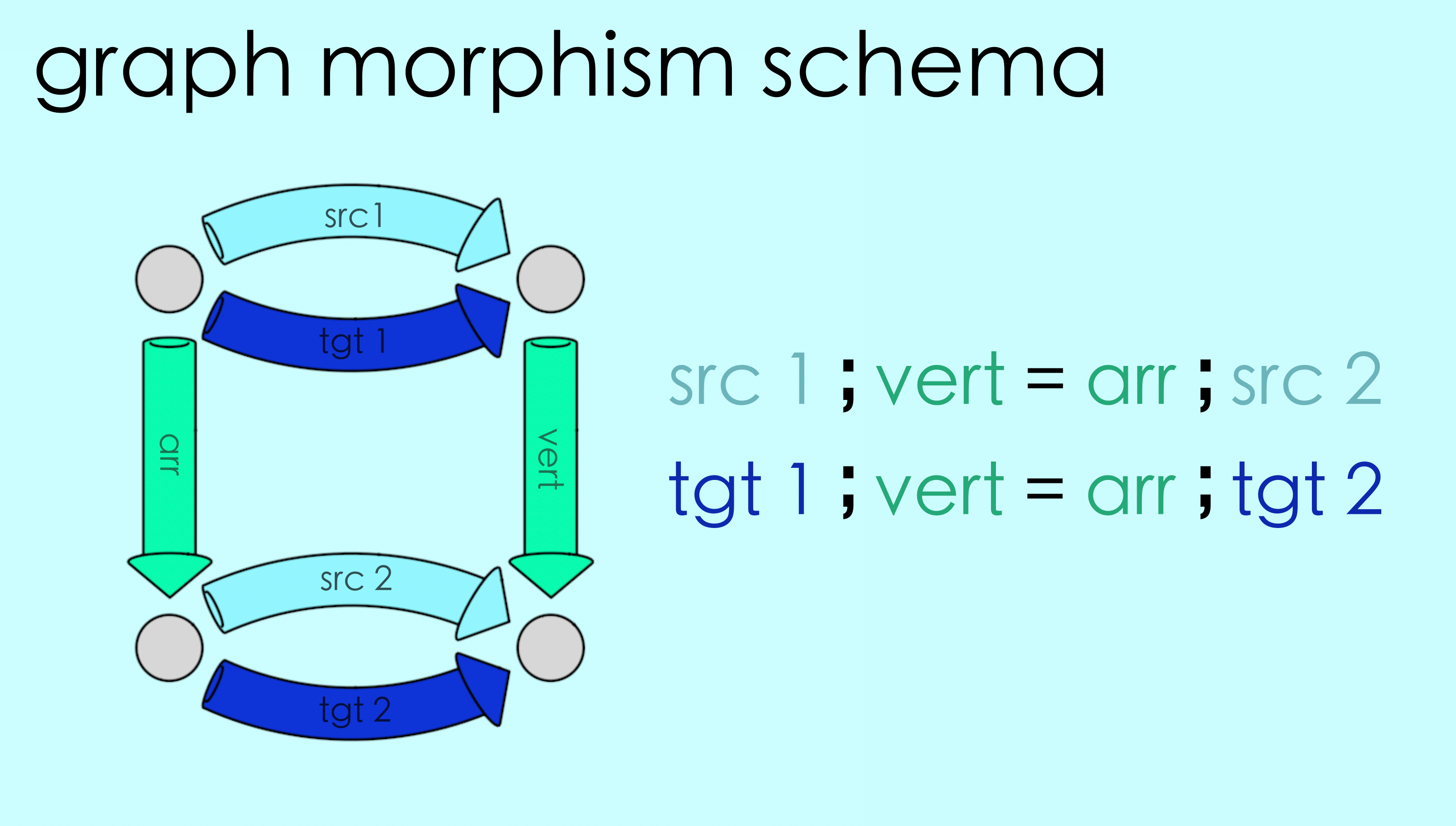
We have once again captured an idea–graph injections–in terms of a schema and some commutativity conditions. But we’re not quite done! In the next section we’ll see that graph injections aren’t the only thing captured by this schema…
5.3 Graph Morphisms#
In Chapter 1 we saw an example of a directed graph which described who’s turn it was to do the dishes. In this account, Paul and Toni originally took turns. Then, eventually, their new roommate Tuco moved in and took over dishes duty. As it turns out, Paul and Toni are both right handed while Tuco is left handed. Thus, there is another directed graph which also accurately describes the chore progression, but now in terms of the handedness of dish-washer.
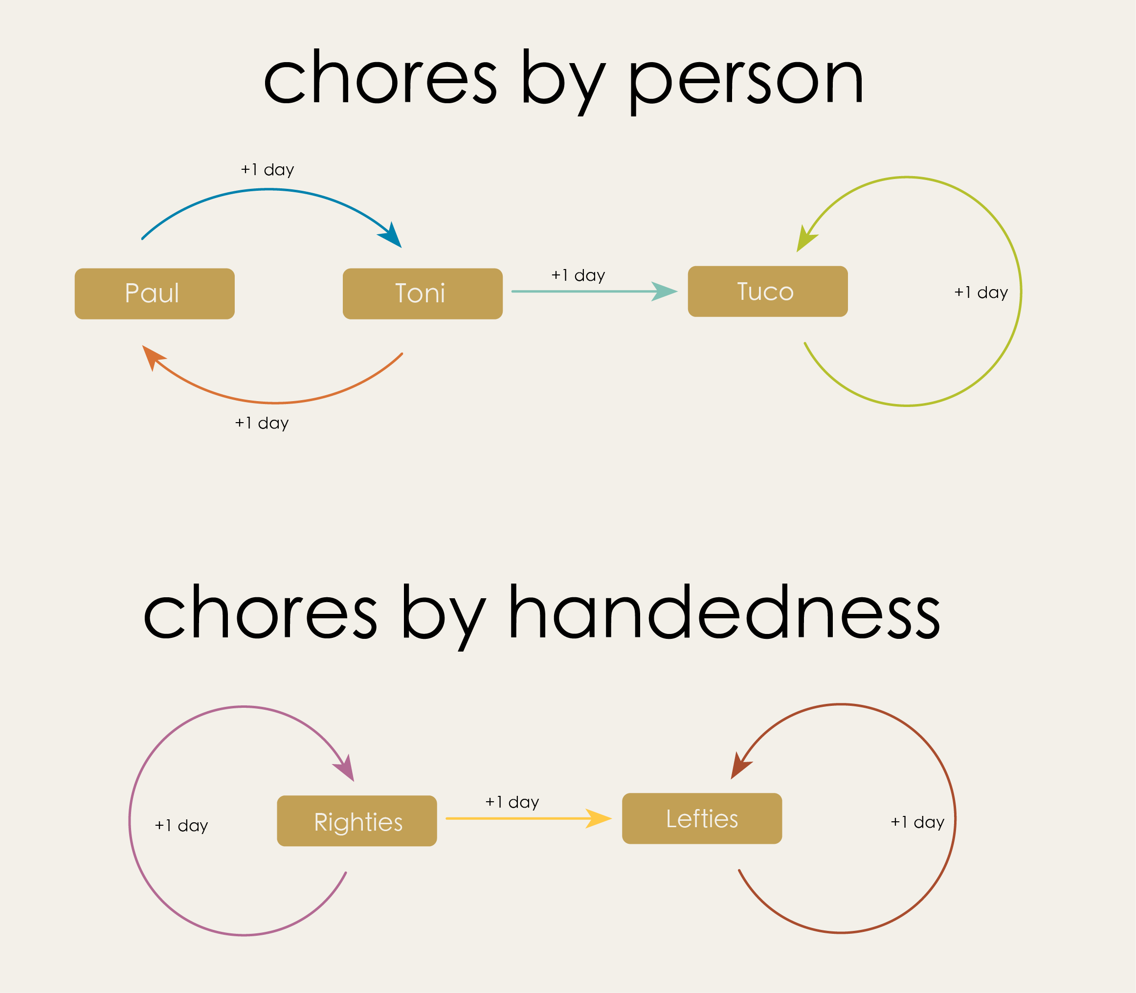
The second model is a “coarse grained” version of the first. It is consistent with the first model but contains fewer details (i.e., it does not tell us which right handed person is doing the dishes at any given moment).
Pause and Ponder
How are these two graphs related?
General graph morphisms#
The coarse-graining we discussed above can be captured by the following way of mapping Graph 1 (Paul, Toni, Tuco) into Graph 2 (Rightie, Leftie):
Coarse graining
Send the
Paulvertex to theRightiesvertexSend the
Tonivertex to theRightiesvertexSend the arrow from
PaultoTonito the self-loop onRightiesSend the arrow from
TonitoPaulto the self-loop onRighties
We call this a “graph morphism”, a way of identifying one graph inside of another that allows for coarse-graining of vertices/arrows. Injections are just a special case of graph morphisms in which there is one-to-one mapping between vertices of Graph 1 and Graph 2, and between arrows of Graph 1 and Graph 2.
Be-as-you-are morphisms#
Every graph instance has a special morphism called “Be-as-you-are” morphism from the graph to itself. True to its name, the be-as-you-are morphism leaves the graph as it is, by sending each vertex to itself and each arrow to itself.
While this morphism may sound quite boring, it is special and is used for saying computationally when two graphs are the same. This special morphism will help us formulate another special graph morphism called isomorphisms for this purpose.
Graph isomorphisms#
Here is something for you to ponder over!
Pause and Ponder
Suppose we have Graph 1 injecting into Graph 2, and Graph 2 also injecting into Graph 1, what can we say about Graph 1 and Graph 2? Here is an aid for your visualization:
Are you convinced that Graph 1 and Graph 2 must have exactly the same number of vertices, the same number of arrows and have the same connectivity? In other words, Graph 1 and Graph 2 are ONE and the SAME for all practical purposes.
Note
In computational terms, we say that Graph 1 and Graph 2 are the same when,
There is a graph morphism from Graph 1 to Graph 2
There is a graph morphism from Graph 2 to Graph 1
For any vertex or arrow in Graph 1, following the morphism from Graph 1 followed by the morphism from Graph 2 results in the same effect as the “be-as-you-are” arrow for Graph 1.
For any vertex or arrow in Graph 2, following the morphism from Graph 2 followed by the morphism from Graph 1 results in the same effect as the “be-as-you-are” arrow for Graph 2.
In the next chapter, we will see that the ability of comparing two graphs and saying if they are the same is quite ubiquitous.
Avoiding dangling edges#
Getting back to general graph morphisms, tt may seem like collapsing parts of the directed graph this way would be an undesirable thing to do. After all, we have to be so careful about breaking a graph, which would violate our DANGLING EDGE CONDITION and ruin any underlying model. Doesn’t coarse-graining our graph pose a similar risk?
It turns out that under the right circumstances, merging parts of a graph won’t actually pose any danger to the integrity of the underlying model.
Let’s consider the dishwashing chores graph morphism we just looked at, but now using generic shapes. We have a morphism from the upper graph to the lower graph.
The result of that morphism looks like this:
Although some of the arrows in the above graph are doubled up, each of them is still pointing to the correct targets and pointing away from the correct sources. The connectivity of the graph is preserved. It turns out that our commutativity condition is the exact condition needed in order to keep the graph intact. For example, observe the closed loops for the sources in this morphism:
Overall, the following schema characterizes all possible graph morphisms:
Of course, this is a very abstract way of thinking about something that is actually relatively simple. Here’s the main idea to keep in mind:
Key idea
A graph morphism is a good way of identifying one graph inside of another. It preserves the connectivity of the domain graph (the graph at which the morphism starts) and may coarse-grain the information.
The value of the abstract view is that it gives AlgebraicJulia a way to work with this idea too. In the following puzzles you will use AlgebraicJulia to help you “count” the number of possible morphisms between pairs of graphs.
Graph morphisms in Algebraic Julia#
Puzzle 3.
We have seen that Graph 1 can be mapped into Graph 2 with the following injection:
How many other morphisms are there from Graph 1 to Graph 2?
We’ve programmed this problem into the executable code below. When you think you know the answer, execute code and see if you and AlgebraicJulia agree.
using Catlab.CategoricalAlgebra, Catlab.Graphs, Catlab.Graphics

Graph1 = Graph()
add_vertices!(Graph1, 2)
add_parts!(Graph1, :E, 2, src=[1,2], tgt=[2,1])


Graph2 = Graph()
add_vertices!(Graph2, 3)
add_parts!(Graph2, :E, 4, src=[1,2,2,3], tgt=[2,3,1,3])

countTheMorphisms = length(homomorphisms(Graph1, Graph2))
Puzzle 3 Solution:
There are three distinct morphisms from Graph 1 to Graph 2; two injections and one way of collapsing the whole graph down to one vertex.
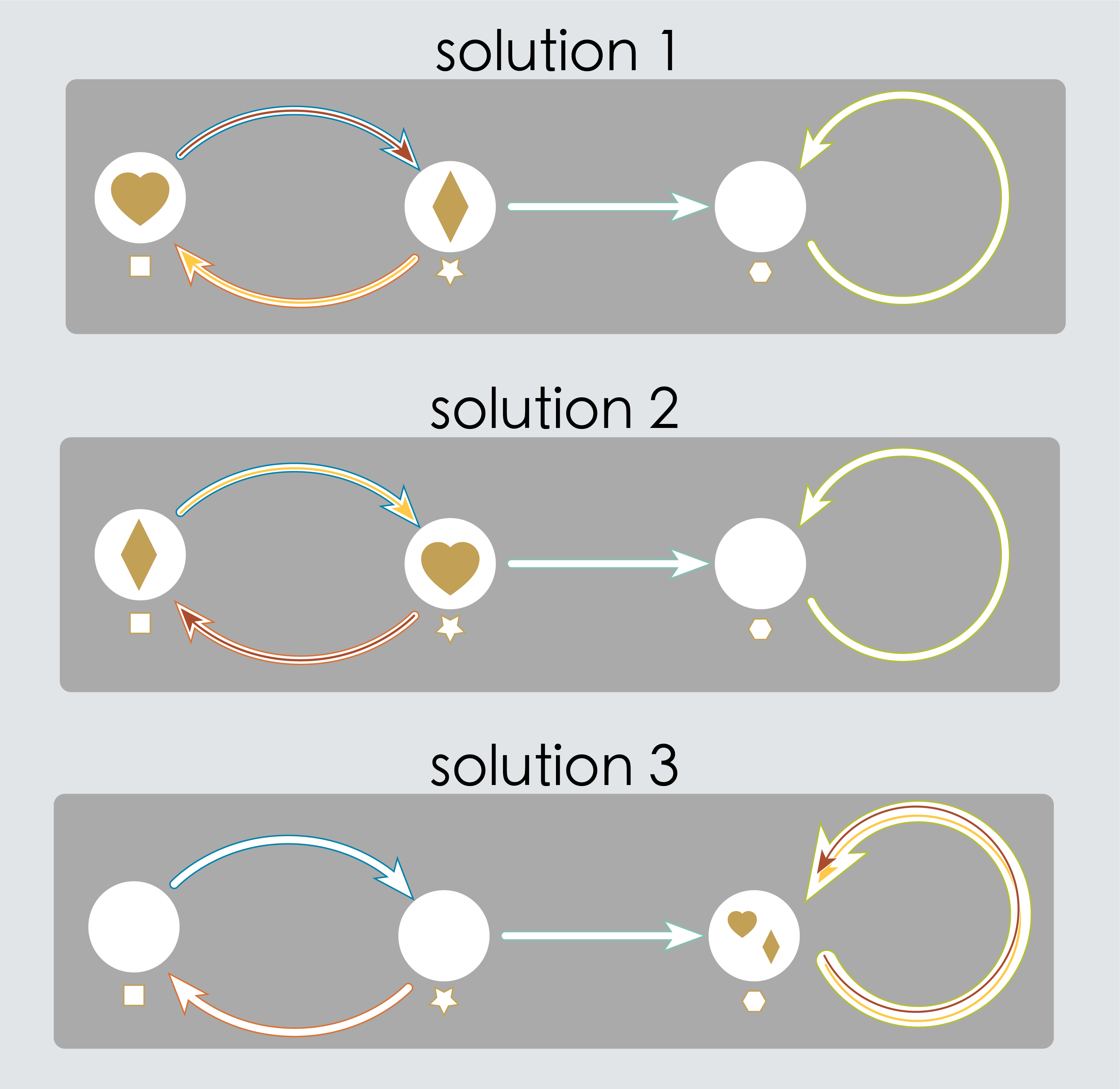
As a human, you look for the answer to this puzzle by reasoning about the shape of the directed graph. AlgebraicJulia looks for its answer by trying to count all of the pairs of vertex maps and arrow maps which complete the commutative squares in the graph morphism schema.
These are very different approaches but they both arrive at the same answer.
Puzzle 4.
How many ways can this triangle be mapped into this hexagon?
Does AlgebraicJulia agree?
hexagon = Graph()
add_vertices!(hexagon, 6)
add_parts!(hexagon, :E, 6, src=[1,2,3,4,5,6], tgt=[2,3,4,5,6,1])

triangle = Graph()
add_vertices!(triangle, 3)
add_parts!(triangle, :E, 3, src=[1,2,3], tgt=[2,3,1])

countTheMorphisms = length(homomorphisms(triangle, hexagon))
Puzzle 4 Solution:
Trick question! There are no ways of mapping the triangle into the hexagon without breaking the DANGLING EDGE CONDITION.
Note how AlgebraicJulia knows when you’ve asked it to find something that doesn’t exist!
Puzzle 5.
What about the other way around? How many ways can this hexagon be mapped into this triangle?
countTheMorphisms = length(homomorphisms(hexagon, triangle))
Puzzle 5 Solution:
Three!
The hexagon can get “doubled up” into the shape of a triangle, and placed into the triangular graph in any of three orientations.
Puzzle 6.
How many ways can the graph on the left into the graph on the right?
Graph3 = Graph()
add_vertices!(Graph3, 2)
add_parts!(Graph3, :E, 2, src= [1,1],tgt= [1,2])

Graph4 = Graph()
add_vertices!(Graph4, 4)
add_parts!(Graph4, :E, 5, src=[1,1,1,1,4], tgt=[1,2,3,4,4])


countTheMorphisms = length(homomorphisms(Graph 3, Graph 4))
Puzzle 6 Solution:
There are five morphisms - three injections and two ways of collapsing to a self-loop
Puzzle 7.
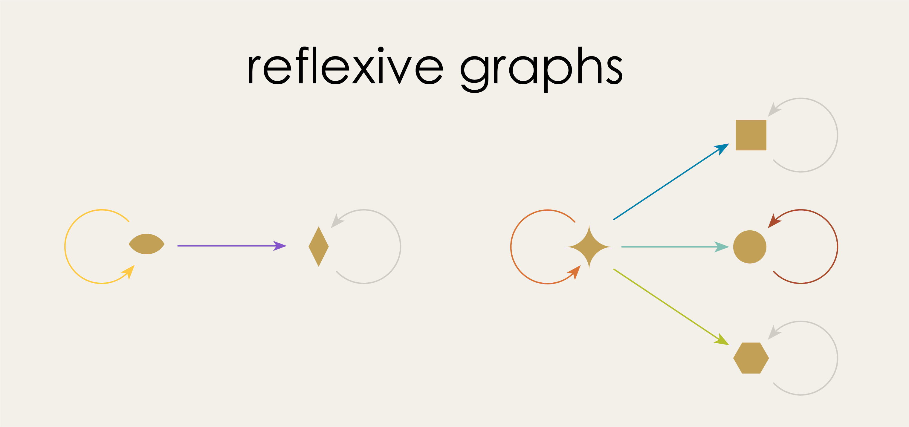
This puzzle is the same as puzzle 6, except in the AlgebraicJulia code below we’ve stipulated that graphs are ReflexiveGraphs instead of DirectedGraphs. This implies the presence of additional self loops (shown in light grey), which changes the number of possible morphisms.
Graph5 = ReflexiveGraph()
add_vertices!(Graph5, 2)
add_parts!(Graph5, :E, 2, src= [1,1],tgt= [1,2])

Graph6 = ReflexiveGraph()
add_vertices!(Graph6, 4)
add_parts!(Graph6, :E, 5, src=[1,1,1,1,4], tgt=[1,2,3,4,4])


countTheMorphisms = length(homomorphisms(Graph 5, Graph 6))
Puzzle 7 Solution:
Seven; Three injections and four maps to self-loops.
Note how AlgebraicJulia succeeds at counting these morphisms correctly. Moreover, it uses the same mechanism as for directed graphs, no need to write specialized code for reflexive graphs.
5.4 The category of instances#
Now that we know what graph morphisms are, we’re ready to move up the last rung in our ladder of abstractions, from “blueprints” (schemas) to “categories!”
Let’s revisit the graph morphism schema and look closely at an instance:
Note how the top of this square contains the data for Graph 1 and the bottom is the data for Graph 2. The overall blueprint represents a morphism of Graph 1 into Graph 2. It almost feels like an arrow pointing from the top to the bottom.
In chapter 3 we introduced ‘chunky arrows’ as a way to hide the messy details of our maps. We will apply the same idea here, defining a new kind of arrow (shaded, light colored on a white background) that encompasses all the details of a graph morphism.
Attention
We know what you’re thinking! “Another kind of arrow?! At another level of abstraction?!”
This is the last one.
Promise. However, note that, we are using the same idea of packing up smaller arrows using chunky arrows.
Geometric vs Schema views#
For us humans, graph morphisms are about the geometric process (Rung 1) of identifying one graph up inside of another. But, our geometric understanding has precise correlation with AlgebraicJulia’s formal representation of graph morphisms using pairs of maps and closed loops (Rung 2 and 3). Thus, we each have our own “language” for describing graph morphisms.
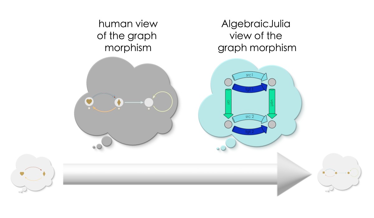
The geometric view is spatial and visual, intuitive for humans to think about. As we observed back in Chapter 0, thinking visually and geometrically about graphs is an excellent way for humans to conceptualize structure. In fact, for the remainder of this book we will only be thinking about graphs and graph morphisms in these natural geometric terms.
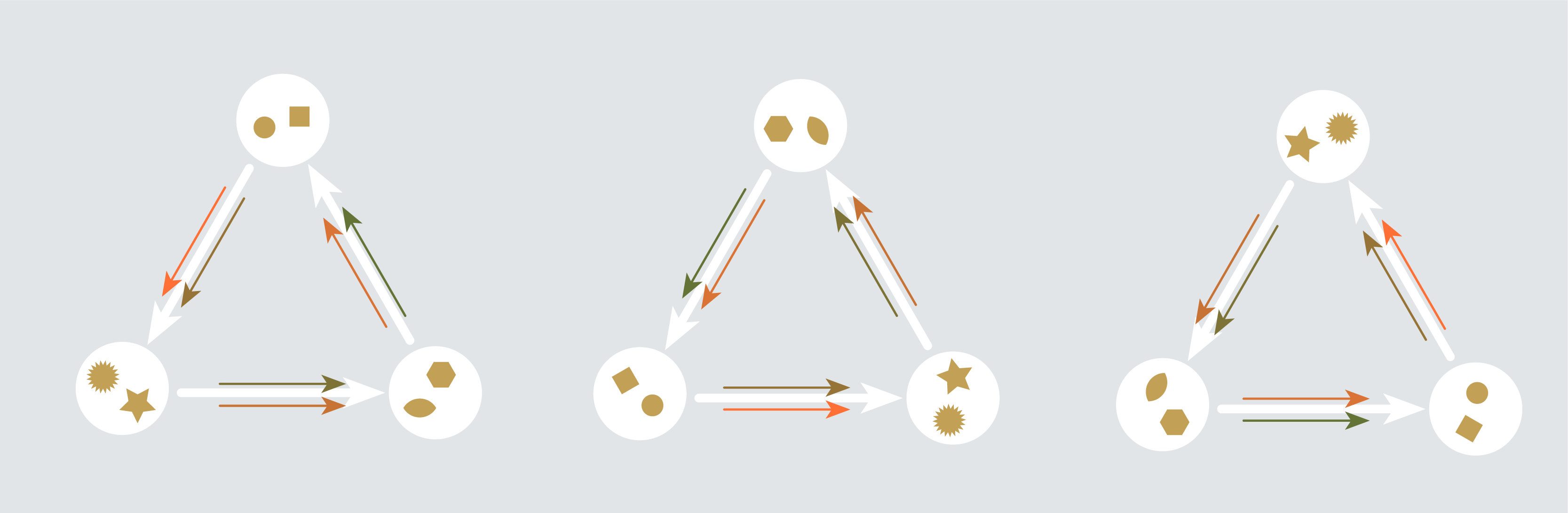
AlgebraicJulia’s view is more abstract but is useful to us because it can be readily worked with in computational terms. Recall puzzle 3 above, where we gave AlgebraicJulia the data of two graphs and asked it to count up all the morphisms between them. AlgebraicJulia correctly found three. Diagrammatically, we depict these morphisms as three distinct arrows going from one graph instance to the other.
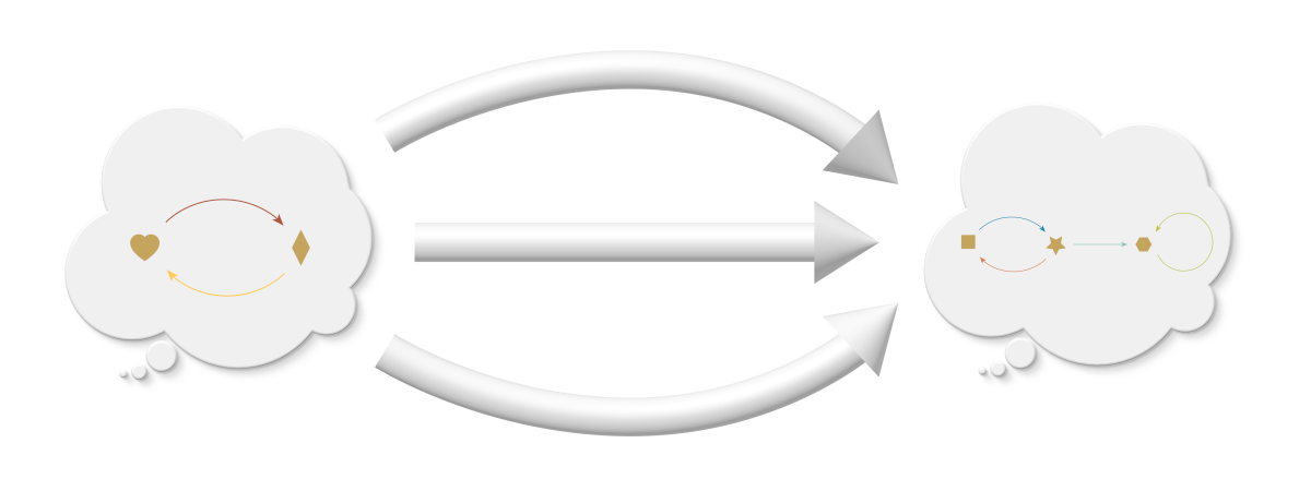
Back to categories#
At the beginning of the chapter we considered the idea of an infinite universe of thought bubbles, each an instance for the given graph schema. We now can say that between those instances are arrows representing morphisms. Just as it was impractical to try to depict all of the instances of a graph schema, it is also impractical to try to depict all the instances of morphisms between two graphs. But in our imagination we can fill in enough of these arrows to appreciate the vast interconnected universe of relationships between graphs. This universe of thought bubbles and arrows is called a category, in this case the “category of instances” for a given schema.
In puzzle 3, when AlgebraicJulia counts three morphisms between a pair of instances, it’s as if it were looking into this category and had the ability to “see” its structure and to retrieve all the arrows that fit our description, like a magic genie that with omniscient access to this universe.
Granted such access, we will next explore this universe and discover a variety of useful patterns that exist here.
5.5 Summary#
In this chapter we have developed the crucial idea of graph morphisms. We have understood this concept from two points of view, the geometric human view and the more formal computational vantage of AlgebraicJulia. The exact correspondence between these views means that if we only think about graphs and graph morphisms geometrically then everything we think can be encoded in AlgebraicJulia!! In the next two chapters we will discover patterns of morphisms that correspond to useful operations like adding, deleting, merging, etc. And we shall see that when we operationalize these patterns with AlgebraicJulia, we end up in a very advantageous position with regards to the DANGLING EDGE CONDITION.
Footnotes and References#
In this chapter and the last we have seen that lot of ideas that can be captured by connecting maps together and then declaring some commutativity conditions. Commutative diagrams are the bread and butter of category theory. We will not explore the general notion of commutativity in much depth here. For a thorough yet elementary introduction to this topic we recommend Lawvere and Schanuel’s Conceptual Mathematics.[1]