Chapter 4: Blueprints - Part II

Note

This book is a work-in-progress! We’d love to learn how we can make it better, especially regarding fixing typos or sentences that are unclear to you. Please consider leaving any feedback, comments, or observations about typos in this google doc.

4.1 Introduction

Let us continue our journey of developing blueprints. In this chapter, we shall move beyond directed graphs, look into other flavors of graphs and how their blueprints are built upon the blueprints of directed graphs.

4.2 Reflexive Graphs (in theory)

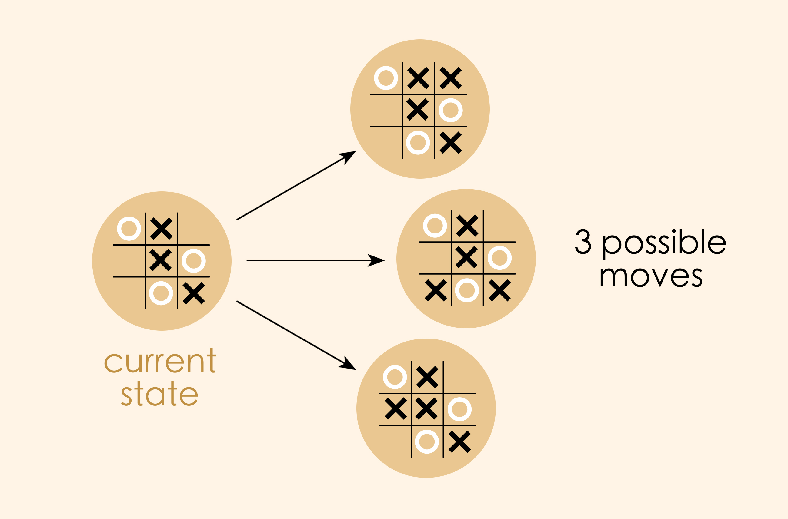
Suppose we were making a directed graph to represent the game of tic-tac-toe, where:

• Vertices are the states of the game

• Arrows are “moves” of the game, going from one state to another.

A piece of our graph would look like this:

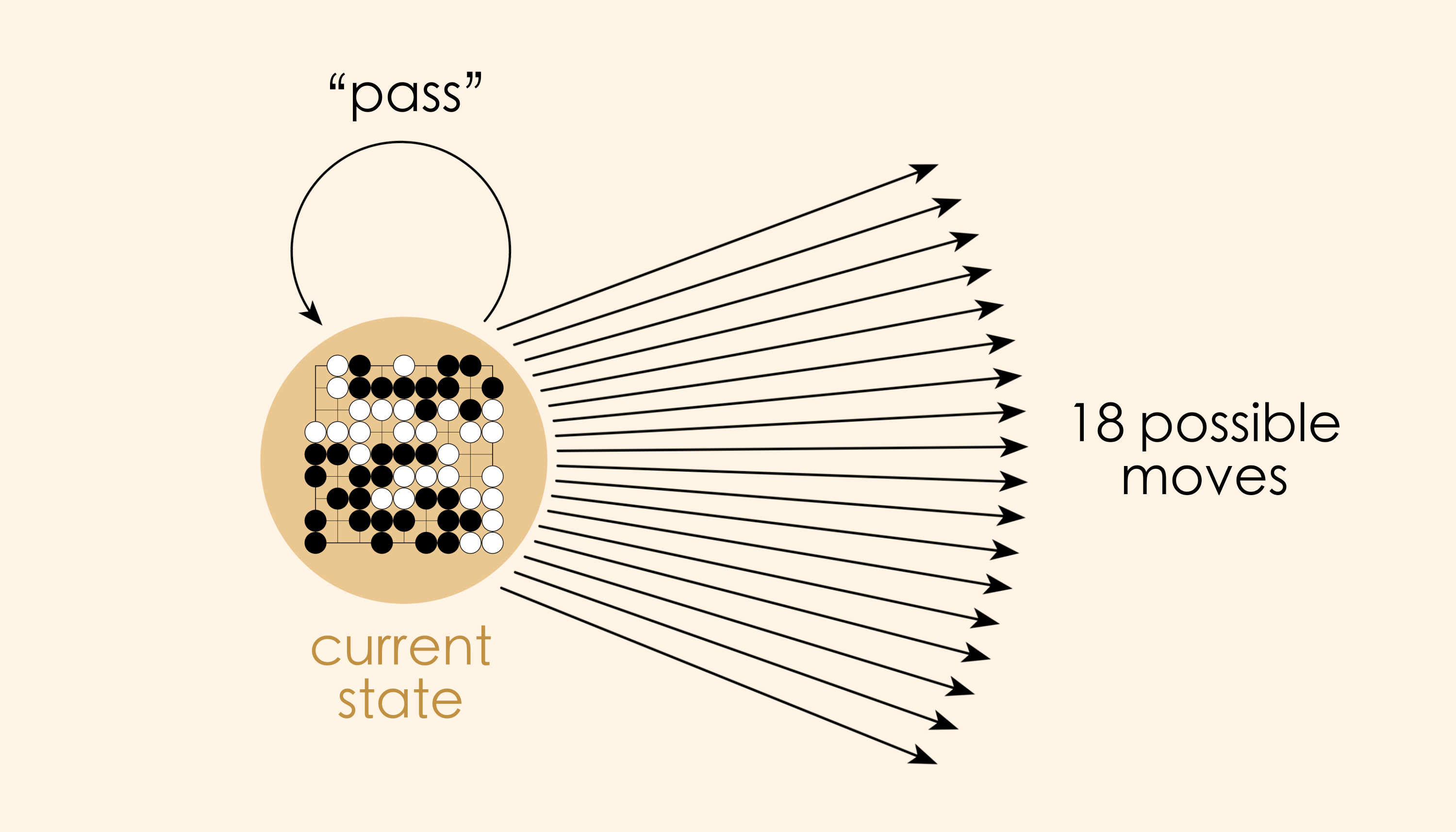
Now let’s imagine doing the same thing for the ancient board game Go. An important thing to know about this game is that the player always has the option to “pass.” That is, one of the available moves on any given turn is to stay in the current state. Thus, every vertex in our graph is going to have one special arrow that loops back on itself.

This actually happens a lot when modeling with directed graphs: we find ourselves wanting every vertex to have a special “self-looping” arrow attached to it. In fact, this happens so frequently that we give these graphs a special name - they’re called “reflexive graphs.” They are widespread and useful. In applied settings they are excellent for geometric applications. Reflexive relationships are prevalent in mathematics (divisibility among the integers, subsets among sets, etc.). And in category theory all structures of interest (preorders, categories, etc.) are reflexive graphs.

Pause and Ponder!

How is the data of a reflexive graph different from the data of a directed graph? How might you communicate the details of a reflexive graph to a computer?

A reflexive graph is simply a directed graph with an added condition that “every vertex has a special self-looping arrow.” This idea can be expressed with a map going from vertices to arrows, where each vertex is connected to its self-looping arrow.

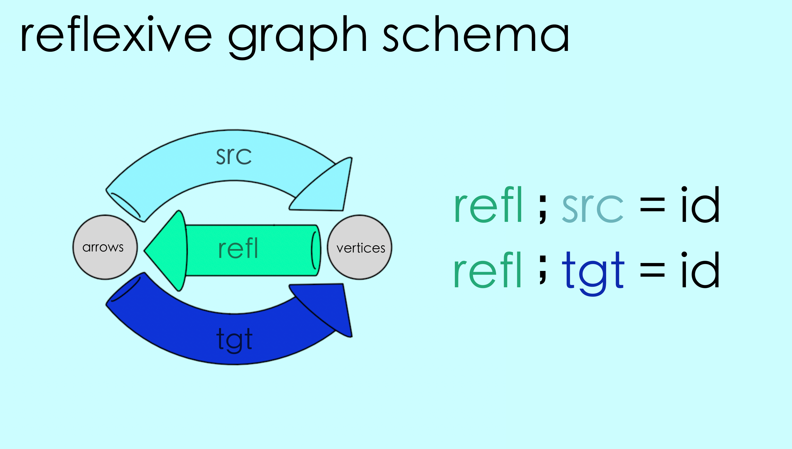
Every reflexive graph has such a map, called its reflexive map or refl. We can combine this reflexive map with the graph’s source and target maps. (Notice that the reflexive map points in the opposite direction, from vertices to arrows.)

Pause and Ponder!

Let your eyes follow the dashed lines around the figure. Do you see any “patterns” in this system of connections?

What can we notice about the above instance? Well, for one thing, in order for an arrow to be the self-loop of a given vertex, it must have that vertex as its source. Another way to look at this is:

The following path always takes you back to where you started:

1. Start from any vertex

2. Follow the reflexive map from this vertex to its self-looping arrow.

3. Continue along the source map from that arrow to it its source vertex.

For example if we start at the heart, the reflexive map takes us to the reddish arrow, and the source map takes us back to the heart:

By the same reasoning, the target map following the reflexive map should always form a closed loop as well.

If we look closely at the maps we indeed see that all such loops are closed:

This closed loop condition turns out to be what it means for a graph to be reflexive graph:

• If every vertex of a graph has a self-loop, then the closed loop condition will be satisfied.

• If the closed loop condition is satisfied, then each vertex of the graph has at least one self-loop.

Pause and Ponder!

Can you convince yourself that the above two bullet points are true?

When we first defined reflexive graphs we had to establish what we meant using semantic ideas like “self-loops” and phrases like “for every vertex…”. We have now found an equivalent way of saying the same thing in terms of maps and whether or not certain paths form closed loops. And “maps and closed loops” are exactly the kind of thing AlgebraicJulia can understand!

Reflexive graphs (in a computer)

Let’s encode a reflexive graph schema in AlgebraicJulia! In order to specify our closed loop condition in a way that a computer can understand we have to convert it into a text expression. Here’s the system we’ll use for writing:

Writing system:

• ; We’ll use a semicolon to sequence paths. So A;B means “path A followed by path B.”

• = We’ll use an equals sign to equate the endpoints of two paths

• id We’ll use this to mean ending up “back where you started.” It refers to the “identity map”, the map equivalent of staying put.

So we can write “the reflexive map followed by the source map takes you back where you started” as:

refl ; src = id

And “the reflexive map followed by the target map takes you back where you started” becomes:

refl ; tgt = id

Equations like this are known as commutativity conditions. These commutativity conditions that the underlying maps must satisfy are also part of the schema. So, schemas are more than directed graphs. Schemas are our fundamental mechanism for encoding things in AlgebraicJulia. Here is the schema for reflexive graphs:

To enter this into AlgebraicJulia we start with the directed graph schema we made earlier and add the refl arrow and our commutativity conditions. (We use compose(X,Y) to mean X ; Y.)

@present ReflexiveGraph <: DirectedGraph begin

  refl::Hom(V,A)

  compose(refl, src) == id(V)
  compose(refl, tgt) == id(V)

end

And that’s how reflexive graphs can be defined in AlgebraicJulia! In the next chapter we’ll see how to put this definition to use.

4.3. Undirected Graphs

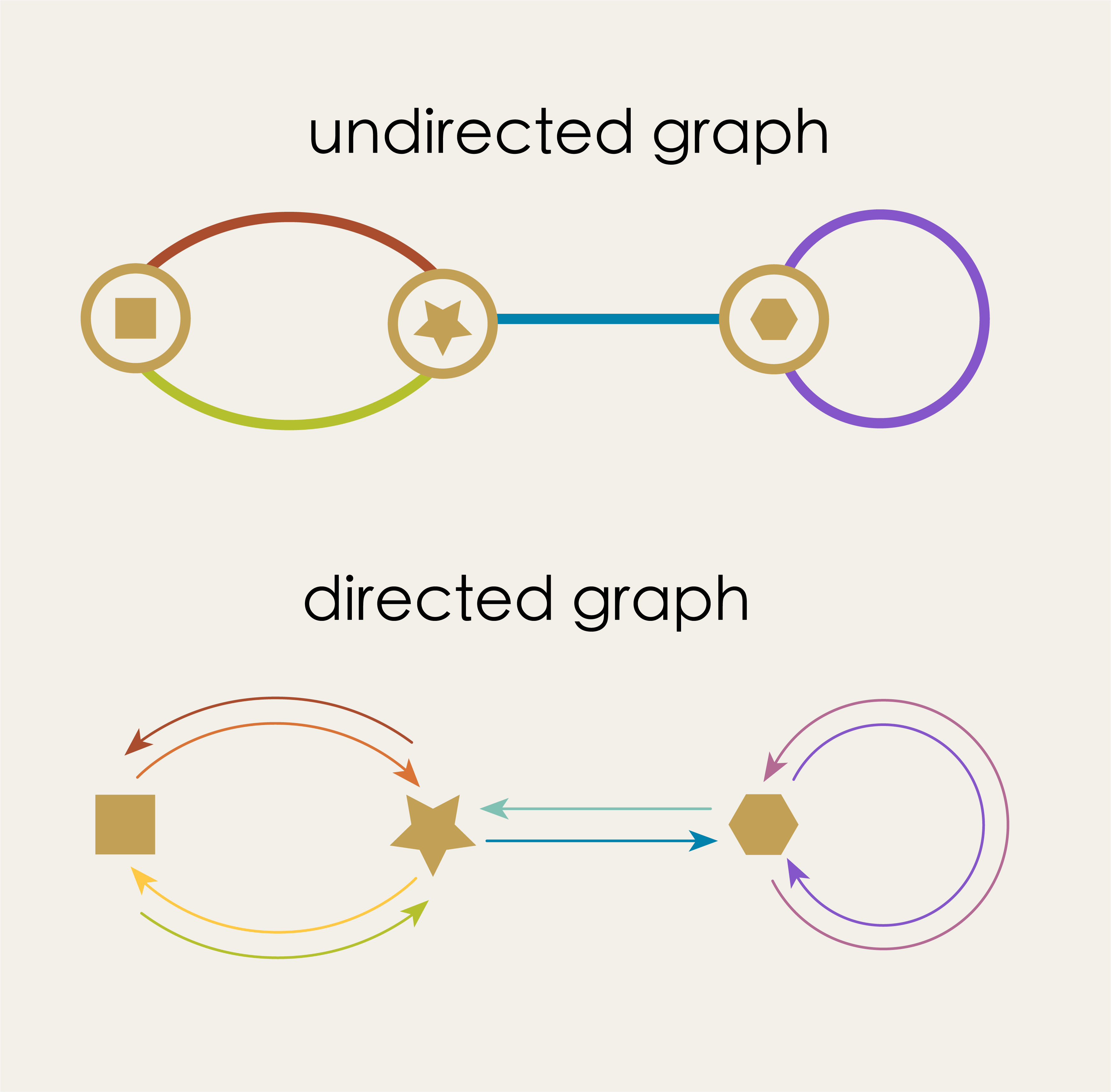
Now let’s return to the question of undirected graphs. Can we design a schema for these? Surprisingly, it turns out that we can think of undirected graphs as special cases of directed graphs.

An arrow in a directed graph is like a one-way street, a unidirectional connection pointing from its source to its target. In an undirected graph, an edge is more like like a two-way street in which the connection is felt mutually in both directions. If we take this “two-way street” analogy literally we can see that every undirected graph is equivalent to a directed graph in which we’ve substituted a pair of opposing arrows in place of each undirected edge.

The directed graph represents the undirected graph if we imagine the opposed arrows just canceling each other out. For this to work, the directed graph must satisfy the condition that “every arrow is associated with a unique partner arrow.” We can express this idea as a map, in which each arrow gets connected to its unique partner:

We call this the inversion map or inv. We can combine this inversion map with the graph’s source and target maps, attaching it as a self-loop.

Notice how the instance data represents a directed graph which in turn represents an undirected graph!

Pause and Ponder!

Let your eyes follow the dashed lines around the figure. Do you see any “patterns” in this system of connections?

What can we notice about the above instance? Well, for one thing, the paired arrows in the directed graph must point in opposite directions. This means that the vertex at which one arrow starts (its source) must be equal to the vertex where its partner arrow lands (its target) and vice versa. We can express this as a closed loop condition.

Comparing two paths

Path 1

1. Start from any arrow in the grey circle

2. Follow the source map from this arrow to its source vertex.

Path 2

1. Start from the same arrow

2. Follow the inversion map to that arrow’s partner

3. Follow the target map from that arrow to its target vertex

Both routes should end up at the same vertex!

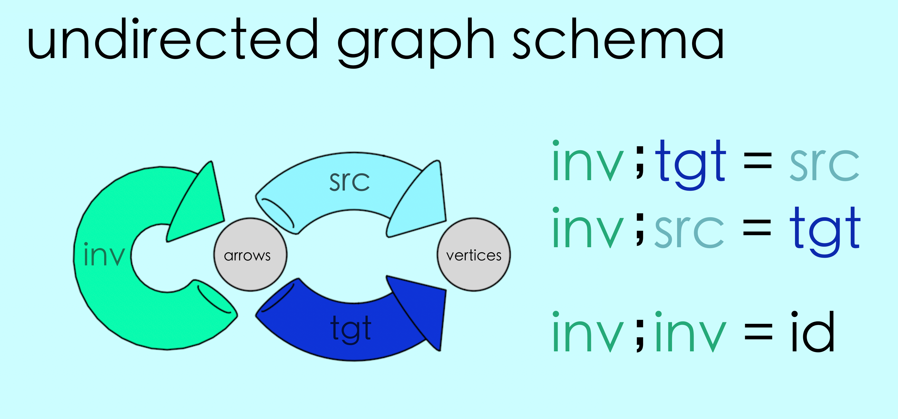
So the commutativity conditions that ensure that partner arrows point in opposite directions are:

inv ; tgt = src

inv ; src = tgt

We also want these partnerships to be unique, meaning we don’t want “cliques” of three, four, five, arrows, each one partnered with the next. To avoid this, each arrow must be its partner’s partner.

inv ; inv = id

Putting it all together, here is the schema for undirected graphs

And here’s how we write this definition in AlgebraicJulia:

@present UndirectedGraph <: DirectedGraph begin
  
  inv::Hom(A,A)

  compose(inv,tgt) == src
  compose(inv,src) == tgt
  
  compose(inv,inv) == id(A)

end

Pause and Ponder!

Consider the difference between your understanding of graphs and AlgebraicJulia’s. For you, this schema might represent a directed or undirected graph. You can interpret it any way you like. Moreover, whatever graph you have in mind may represent still other ideas like chores and mood swings. But for AlgebraicJulia there is no interpretation. Ideas are phrased exclusively in terms of schemas, maps and commutativity conditions. It has no idea what any of this “means” to you.

We use thought bubbles to indicate these interpretations, signalling that the meaning of any instance is an idea that exists only the in mind of the programmer.

4.4 Other kinds of schemas

In this chapter we have used schemas and commutativity conditions to look at a few different flavors of graphs. But the framework we have developed here can actually be extended beyond just graphs, to an extraordinary variety of elaborate and useful concepts.

Indeed, one of the profound offerings of AlgebraicJulia is the sheer number of mathematical abstractions it can handle in terms of schemas.

In this final section we offer a brief glimpse at some more powerful models and ideas that are also captured by this framework.

DISCLAIMER: It is out of scope to go into any detail on the following schemas. We mention them here, in passing, only to give some sense of the possibilities with AlgebraicJulia.

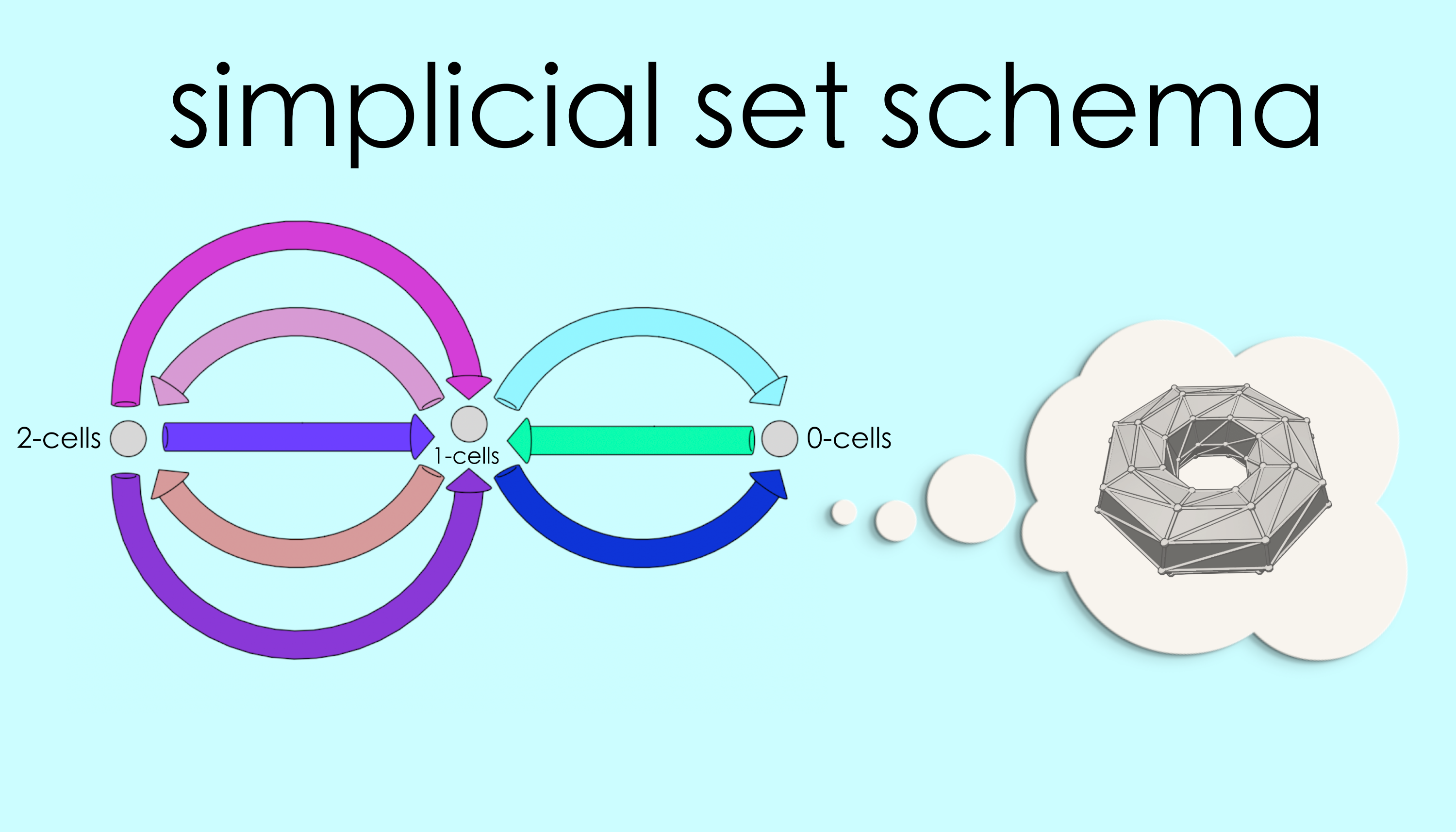
Simplicial sets

We can generalize reflexive graphs to higher dimensions using schemas. The result is one of the algebraic topologist’s favorite tools: simplicial sets. Ordinary graphs connect 0-dimensional vertices using 1-dimensional lines. With simplicial sets we can also attach 2-dimensional triangles, building up triangulated surfaces. Going up another dimension we can attach 3-dimensional tetrahedra to make solid figures. And so on.

For the mathematician, simplicial sets are useful because they turn geometry into algebra: a simplicial triangulation of a topological space is a combinatorial object that can be reasoned about. For the applied scientist, simplicial sets may be useful as a way of 3D modeling, as we’ll see in Chapter 8. Finally, in AlgebraicJulia, simplicial sets are practical because all of the rules for how different parts must attach can be fully captured with a few commutativity conditions.

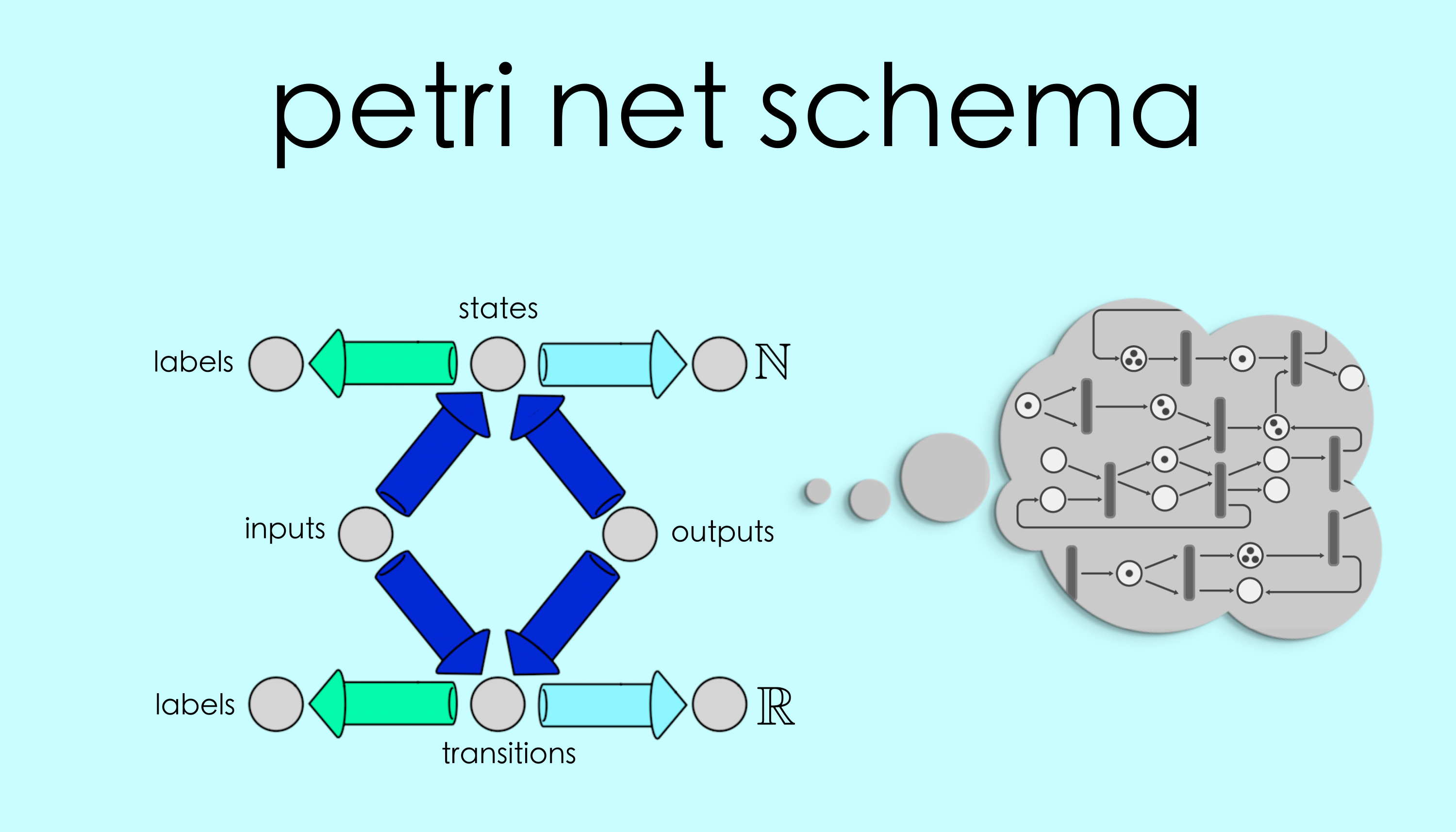
Petri nets

On the more “applied” side, we have the example of Petri nets, a sophisticated modeling system for the analysis of concurrent systems. It was developed by German computer scientist Carl Adam Petri in the 1960’s, whose goal was to provide a system that could model parallel processes, synchronization and resource sharing. Petri nets provide a modeling tool that is suitable for a wide variety of systems, from chemical reactions to business management logistics.

It’s important to note that Petri nets were developed by practitioners, not mathematicians. The system was born from necessity, designed to fill a utility gap in other approaches to modeling. But because Carl Petri gave the system an exact mathematical definition for its execution semantics we are able to represent Petri nets in terms of schemas and work with them in AlgebraicJulia.

AlgebraicJulia’s implementation of Petri nets is called AlgebraicPetri.jl.[1] Documentation can be found here along with several examples of scientific models, including population dynamics, epidemiological models and enzyme reactions.

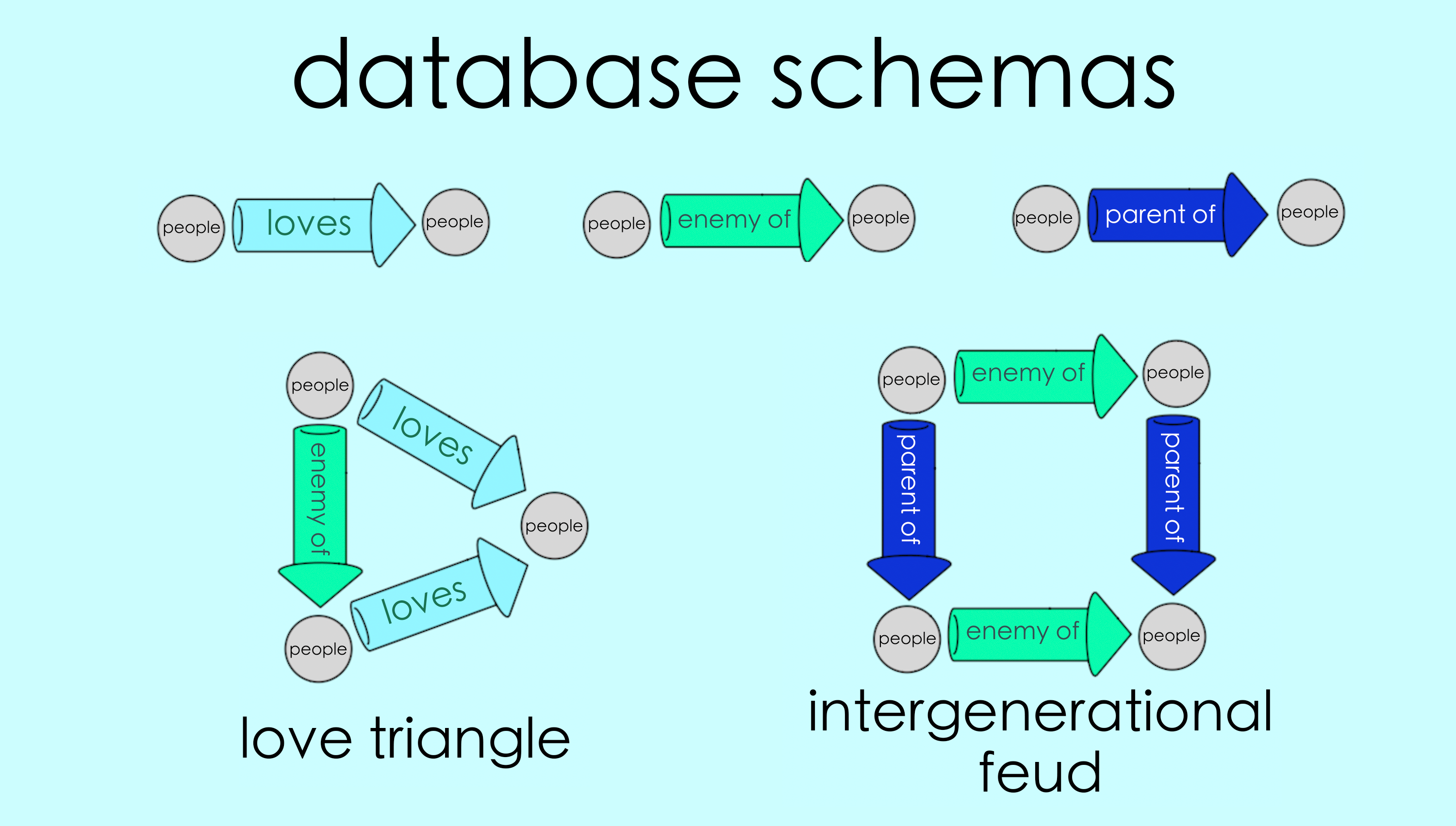
Databases

The whole concept of a schema originally comes from database theory. We can think of the underlying connections in a schema as linked data. For example the grey circles may represent a database of ‘people’ and a given arrow may repesent a tabulated relationship between those people (Who loves whom? Who is the enemy of whom? etc.) Structuring a query on that database is then just building a schema to define new relationships in terms of existing ones.

Data often gets corrupted when transferred between contexts, a major issue in database management. Data corruption is a kind of analog for our DANGLING EDGE CONDITION on graphs. And in the same way that AlgebraicJulia will allow us to use high level abstractions to resolve our dangling edge problems, there are other category theoretic techniques for data migration that offer a canonical way of migrating data that automatically takes care of various annoying edge conditions. See the paper Functorial Data Migration[2] for details.

4.5 Summary

In this chapter we have developed the concept of a schema, a versatile data structure and the principal way to define things in AlgebraicJulia. In the next chapter we will put this idea to a specific use, characterizing a certain kind of graph relationship as a schema. In subsequent chapters that relationship will give us a way to manipulate graphs without having to worry about the DANGLING EDGE CONDITION.

Footnotes and References

---

[1]

AlgebraicPetri.jl Documentation. https://algebraicjulia.github.io/AlgebraicPetri.jl/dev/.

[2]

David I. Spivak. “Functorial data migration”. Information and Computation, Volume 217, 2012, Pages 31-51, ISSN 0890-5401, https://doi.org/10.1016/j.ic.2012.05.001. https://arxiv.org/abs/1009.1166.